Determining Trade Union Status

2020-09-02 on Data science, Machine learning, Python, Commerce, Transport

This Project deals with implementation of different models and doing preprocessing with the data in order to compare the results and performance of different models. Weapplied statistical techniques to see which model is performing best. In this project we will create a binary classifier which will predict that either the data scientist will remaina USDU member or not.

Reading data for preprocessing

TRAIN.csv

	gender	Management	USAcitizen	Married	MonthsInUnion	ContinuingEd	FeatureA	Connectivity	FeatureC	FeatureD	FeatureE	FeatureF	FeatureG	FeatureB	DuesFrequency	PaperlessBilling	PaymentMethod	MonthlyDues	TotalDues
0	Male	0	No	No	26	Yes	No	Fiber optic	No	Yes	No	No	Yes	No	Month-to-month	Yes	Electronic check	86	2147
1	Female	0	Yes	No	34	Yes	Yes	Fiber optic	No	No	Yes	No	Yes	Yes	Month-to-month	Yes	Electronic check	100	3415
2	Male	0	No	No	1	Yes	No	Fiber optic	No	No	No	No	No	No	Month-to-month	Yes	Electronic check	70	70
3	Male	1	Yes	No	1	Yes	No	Fiber optic	No	No	No	No	No	No	Month-to-month	No	Mailed check	71	71
4	Male	1	Yes	No	62	Yes	Yes	Fiber optic	No	Yes	Yes	No	Yes	Yes	One year	Yes	Electronic check	104	6383

Test_Data

	gender	Management	USAcitizen	Married	MonthsInUnion	ContinuingEd	FeatureA	Connectivity	FeatureC	FeatureD	FeatureE	FeatureF	FeatureG	FeatureB	DuesFrequency	PaperlessBilling	PaymentMethod	MonthlyDues	TotalDues
DS_ID
10000	Male	0	Yes	No	1	No	Maryville	DSL	No	Yes	No	No	No	No	Month-to-month	Yes	Electronic check	30	30
10001	Female	0	No	No	34	Yes	No	DSL	Yes	No	Yes	No	No	No	One year	No	Mailed check	57	1890
10002	Female	0	No	No	2	Yes	No	DSL	Yes	Yes	No	No	No	No	Month-to-month	Yes	Mailed check	54	108
10003	Female	0	No	No	45	No	Maryville	DSL	Yes	No	Yes	Yes	No	No	One year	No	Bank transfer (automatic)	42	1841
10004	Male	0	No	No	2	Yes	No	Fiber optic	No	No	No	No	No	No	Month-to-month	Yes	Electronic check	71	152

TRAIN.csv “LeftUnion”

	LeftUnion
0	No
1	No
2	No
3	Yes
4	Yes

Train and Test Split

Doing Train and Test Split between data. It involves importing a function from scikit learn librarywhich can perform this task very easily. Now doing Train and Test Split between data. So that we will apply all the preprocessing on train data but not test data. Otherwise our model will get prone to data leakage and it will perform worse in production when newdata arrives.

	gender	Management	USAcitizen	Married	MonthsInUnion	ContinuingEd	FeatureA	Connectivity	FeatureC	FeatureD	FeatureE	FeatureF	FeatureG	FeatureB	DuesFrequency	PaperlessBilling	PaymentMethod	MonthlyDues	TotalDues
0	Male	0	Yes	Yes	2	Yes	No	Fiber optic	No	No	No	No	No	No	Month-to-month	No	Mailed check	70	144
1	Female	0	No	No	16	Yes	No	DSL	No	Yes	No	Yes	No	No	Month-to-month	Yes	Mailed check	54	834
2	Male	1	No	No	7	Yes	Yes	Fiber optic	No	No	No	No	No	No	Month-to-month	No	Mailed check	74	545
3	Male	0	No	No	26	Yes	No	Fiber optic	No	Yes	No	No	Yes	No	Month-to-month	Yes	Electronic check	86	2147
4	Male	0	No	No	2	Yes	No	DSL	No	No	No	No	No	No	Month-to-month	No	Mailed check	45	75

y_train

	LeftUnion
0	No
1	Yes
2	Yes
3	No
4	Yes

Merge data By label

X_train and y_train

	gender	Management	USAcitizen	Married	MonthsInUnion	ContinuingEd	FeatureA	Connectivity	FeatureC	FeatureD	FeatureE	FeatureF	FeatureG	FeatureB	DuesFrequency	PaperlessBilling	PaymentMethod	MonthlyDues	TotalDues	LeftUnion
0	Male	0	Yes	Yes	2	Yes	No	Fiber optic	No	No	No	No	No	No	Month-to-month	No	Mailed check	70	144	No
1	Female	0	No	No	16	Yes	No	DSL	No	Yes	No	Yes	No	No	Month-to-month	Yes	Mailed check	54	834	Yes
2	Male	1	No	No	7	Yes	Yes	Fiber optic	No	No	No	No	No	No	Month-to-month	No	Mailed check	74	545	Yes
3	Male	0	No	No	26	Yes	No	Fiber optic	No	Yes	No	No	Yes	No	Month-to-month	Yes	Electronic check	86	2147	No
4	Male	0	No	No	2	Yes	No	DSL	No	No	No	No	No	No	Month-to-month	No	Mailed check	45	75	Yes

X_test And y_test

	gender	Management	USAcitizen	Married	MonthsInUnion	ContinuingEd	FeatureA	Connectivity	FeatureC	FeatureD	FeatureE	FeatureF	FeatureG	FeatureB	DuesFrequency	PaperlessBilling	PaymentMethod	MonthlyDues	TotalDues	LeftUnion
0	Male	0	Yes	No	53	Yes	No	Dial-in	Maryville	Maryville	Maryville	Maryville	Maryville	Maryville	Two year	No	Credit card (automatic)	20	1110	No
1	Male	1	No	No	52	No	Maryville	DSL	No	Yes	No	No	Yes	Yes	Month-to-month	Yes	Electronic check	49	2551	Yes
2	Female	1	No	No	1	Yes	No	Fiber optic	No	No	No	No	Yes	No	Month-to-month	No	Electronic check	78	78	Yes
3	Male	1	No	No	56	Yes	Yes	Fiber optic	No	No	Yes	No	Yes	Yes	Month-to-month	Yes	Electronic check	101	5594	No
4	Female	0	No	No	3	Yes	No	DSL	No	No	No	No	Yes	No	Month-to-month	Yes	Electronic check	54	140	No

NaN values Check

Checking For Nan values in the dataset column wise. Because we have to remove the nan values before fitting out the ML model on data.For that purpose we are creating a function named check_nan() in which we are passing a dataframe as an argument. It gives us output telling the no of NaN values.

gender              0
Management          0
USAcitizen          0
Married             0
MonthsInUnion       0
ContinuingEd        0
FeatureA            0
Connectivity        0
FeatureC            0
FeatureD            0
FeatureE            0
FeatureF            0
FeatureG            0
FeatureB            0
DuesFrequency       0
PaperlessBilling    0
PaymentMethod       0
MonthlyDues         0
TotalDues           0
LeftUnion           0
dtype: int64

gender              0
Management          0
USAcitizen          0
Married             0
MonthsInUnion       0
ContinuingEd        0
FeatureA            0
Connectivity        0
FeatureC            0
FeatureD            0
FeatureE            0
FeatureF            0
FeatureG            0
FeatureB            0
DuesFrequency       0
PaperlessBilling    0
PaymentMethod       0
MonthlyDues         0
TotalDues           0
LeftUnion           0
dtype: int64

gender              0
Management          0
USAcitizen          0
Married             0
MonthsInUnion       0
ContinuingEd        0
FeatureA            0
Connectivity        0
FeatureC            0
FeatureD            0
FeatureE            0
FeatureF            0
FeatureG            0
FeatureB            0
DuesFrequency       0
PaperlessBilling    0
PaymentMethod       0
MonthlyDues         0
TotalDues           0
dtype: int64

Counting unique values:

Here we are counting unique values for every column in the dataset. For that purpose we again created a function named count_unique() taking dataframe column name as an input.

Checking dataset columns

Yes    338
No     331
Name: USAcitizen, dtype: int64

Binary unique values

No     464
Yes    205
Name: Married, dtype: int64
Yes    602
No      67
Name: ContinuingEd, dtype: int64
Yes    379
No     290
Name: PaperlessBilling, dtype: int64

Encoding

Here we are also encoding our categorical values into binary format so that our machine learning model doesn’t generate any type of error while fitting on data.

	gender	Management	USAcitizen	Married	MonthsInUnion	ContinuingEd	FeatureA	Connectivity	FeatureC	FeatureD	FeatureE	FeatureF	FeatureG	FeatureB	DuesFrequency	PaperlessBilling	PaymentMethod	MonthlyDues	TotalDues	LeftUnion
0	1	0	1	1	2	1	No	Fiber optic	No	No	No	No	No	No	Month-to-month	0	Mailed check	70	144	No
1	0	0	0	0	16	1	No	DSL	No	Yes	No	Yes	No	No	Month-to-month	1	Mailed check	54	834	Yes
2	1	1	0	0	7	1	Yes	Fiber optic	No	No	No	No	No	No	Month-to-month	0	Mailed check	74	545	Yes
3	1	0	0	0	26	1	No	Fiber optic	No	Yes	No	No	Yes	No	Month-to-month	1	Electronic check	86	2147	No
4	1	0	0	0	2	1	No	DSL	No	No	No	No	No	No	Month-to-month	0	Mailed check	45	75	Yes

Plotting Histogram

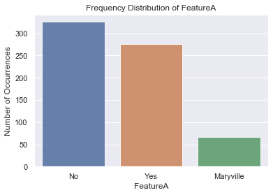
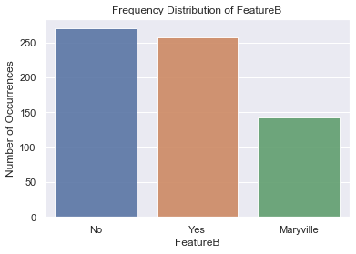
Below we are using matplotlib for Plotting of Histogram. This is used for checking the frequency distribution of different values inside a column or feature. Each column is a different unique feature for our model. As we can see from the output there are 3 labels Yes, No and Maryville.We are plotting for FeatureA and FeatureB.

Non binary unique values

No           326
Yes          276
Maryville     67
Name: FeatureA, dtype: int64
No           270
Yes          257
Maryville    142
Name: FeatureB, dtype: int64
No           308
Yes          219
Maryville    142
Name: FeatureC, dtype: int64
No           290
Yes          237
Maryville    142
Name: FeatureD, dtype: int64
No           285
Yes          242
Maryville    142
Name: FeatureE, dtype: int64
No           336
Yes          191
Maryville    142
Name: FeatureF, dtype: int64
Yes          274
No           253
Maryville    142
Name: FeatureG, dtype: int64
Fiber optic    300
DSL            227
other           92
Dial-in         50
Name: Connectivity, dtype: int64
Month-to-month    355
Two year          160
One year          154
Name: DuesFrequency, dtype: int64
Electronic check             231
Mailed check                 157
Credit card (automatic)      145
Bank transfer (automatic)    136
Name: PaymentMethod, dtype: int64

One hot Encoding:

Doing One hot Encoding for those columns which are containing non binary values. One hot encoding simple converts the values between 0’s and 1’s e.g. 0000001 etc. We use one hotencoding in order to convert our categorical feature column into numeric columns so that modelcan easily do learning. For this purpose we created a function named encode_nb() which is taking 3 arguments. 1 is dataframe, 2nd is the column name and 3rd is the prefix that we wantin the name of every new column.

	gender	Management	USAcitizen	Married	MonthsInUnion	ContinuingEd	PaperlessBilling	MonthlyDues	TotalDues	LeftUnion	...	conn_Dial-in	conn_Fiber optic	conn_other	dues_F_Month-to-month	dues_F_One year	dues_F_Two year	pay_M_Bank transfer (automatic)	pay_M_Credit card (automatic)	pay_M_Electronic check	pay_M_Mailed check
0	1	0	1	1	2	1	0	70	144	No	...	0	1	0	1	0	0	0	0	0	1
1	0	0	0	0	16	1	1	54	834	Yes	...	0	0	0	1	0	0	0	0	0	1
2	1	1	0	0	7	1	0	74	545	Yes	...	0	1	0	1	0	0	0	0	0	1
3	1	0	0	0	26	1	1	86	2147	No	...	0	1	0	1	0	0	0	0	1	0
4	1	0	0	0	2	1	0	45	75	Yes	...	0	0	0	1	0	0	0	0	0	1

5 rows × 42 columns

Nan values in every column in The Dataset

Nan values in every column in The Testset

Nan values in every row.

0      0
1      0
2      0
3      0
4      0
      ..
664    0
665    0
666    0
667    0
668    0
Length: 669, dtype: int64

Plotting and Visualization

Box and whisker plot:

Doing Box and whisker plot for Checking the availability of outliers in the code. The outliers are simply unwanted values in the code that can generate bias if not removed. We are using aseaborn library for plotting Box and whisker plot. Box and whisker plot. Below we are also checking no of unique values for MonthlyDues and TotalDues features.

detecting outlier

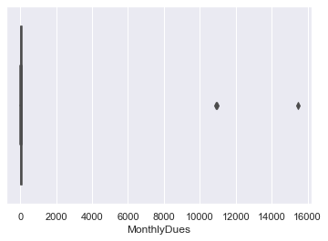
certainly there are outliers Unique MonthlyDues

array([   70,    54,    74,    86,    45,    90,    25,    20,    75,
          94,    60,    79,   111,   100,    69,    85,    76,   104,
         103,    71,    46,    84,   114,    78,   110,   106,    89,
          95,    81,    97,    44,    55,    80,   115,    91,    50,
         109,   108,   112,    67,    56,    53,    24,    64,    99,
          77,    29,    31,   116,   101,    88,    72,    19,    83,
          36,    30,    92,    93,    41,   105,    82,    66,    49,
          26,    21,    58,    98,    51,    68,    96,    34,   113,
          73,   102, 10878,   107,    48,    40, 15453,    61,    65,
          87,    35,    18,    62, 10938,    57,   119,    42])

Unique TotalDues

array(['144', '834', '545', '2147', '75', '145', '248', '25', '952',
       '1129', '1608', '3036', '171', '5565', '70', '7512', '5201', '69',
       '1350', '152', '3467', '4108', '20', '5538', '1975', '1993', '46',
       '5982', '7939', '2840', '68', '855', '1832', '7535', '3650',
       '4513', '2258', '7041', '4614', '3106', '400', '303', '5879',
       '143', '2684', '52', '2018', '573', '563', '2861', '5657', '457',
       '93', '4246', '2614', '4307', '605', '320', '271', '7334', '169',
       '311', '2920', '267', '6938', '470', '7931', '4915', '369', '7796',
       '832', '5000', '2387', '202', '1150', '1208', '1733', '863',
       '1391', '5648', '906', '6442', '3369', '1464', '2708', '2866',
       '8004', '1204', '302', '73', '3632', '196', '3777', '1759', '265',
       '227', '926', '7159', '8425', '4113', '220', '6521', '3173', '19',
       '5213', '1799', '831', '#VALUE!', '261', '2296', '2352', '244',
       '6414', '1169', '476', '7509', '1929', '4698', '1648', '1009',
       '4179', '321', '481', '6083', '1134', '2549', '3211', '255',
       '1381', '3230', '454', '3674', '463', '5013', '3415', '988', '339',
       '4052', '590', '7298', '4965', '6683', '7083', '429', '1212',
       '163', '372', '4689', '621', '5064', '4641', '161', '1314', '1017',
       '3822', '119', '530', '1291', '78', '1521', '1306', '6633', '1238',
       '368', '5031', '29', '1206', '8405', '1527', '81', '134', '744',
       '7554', '3942', '256', '5038', '425', '1395', '1601', '6069',
       '1368', '5731', '1126', '2897', '2821', '7752', '801', '4520',
       '5914', '1171', '1269', '3773', '2931', '2570', '4117', '6591',
       '129', '541', '2263', '3545', '296', '1682', '3858', '1346', '111',
       '451', '3029', '498', '4925', '2245', '6373', '232', '4805',
       '7904', '80', '3883', '1741', '1523', '6735', '2094', '5222',
       '204', '4946', '1597', '2964', '5045', '2398', '1994', '7406',
       '867', '42', '3605', '857', '59', '2110', '245', '865', '4017',
       '1626', '1664', '406', '899', '7031', '5958', '37', '1475', '1264',
       '6046', '219', '5481', '5154', '6393', '6510', '738', '1862',
       '1734', '773', '1125', '4484', '6945', '4009', '1399', '3379',
       '1284', '5770', '332', '2910', '250', '36', '5318', '3510', '7099',
       '4054', '5436', '2388', '1752', '1724', '4304', '464', '1622',
       '756', '3626', '4738', '1410', '434', '5175', '4751', '2509',
       '382', '43', '1629', '4349', '8110', '5681', '92', '1173', '5151',
       '390', '3870', '4542', '7062', '4084', '4754', '94', '6230',
       '4684', '3243', '297', '35', '71', '6980', '564', '48', '158',
       '4665', '617', '294', '453', '5265', '7895', '5826', '947', '5937',
       '44', '6688', '3638', '2724', '79', '7962', '403', '5818', '4056',
       '535', '30', '34', '2239', '4859', '3205', '2443', '3266', '579',
       '7726', '1398', '3067', '5720', '1743', '4992', '6589', '279',
       '6558', '2511', '1461', '1802', '299', '341', '2596', '1725', '74',
       '503', '4677', '696', '91', '522', '1821', '1818', '24', '497',
       '243', '132', '7338', '1320', '32', '663', '3442', '1188', '5043',
       '2586', '1425', '2453', '1531', '123', '1505', '897', '2169',
       '815', '542', '1718', '2722', '6033', '2235', '230', '8313', '521',
       '3046', '235', '8093', '1146', '4817', '679', '3682', '2680',
       '6126', '280', '3646', '1327', '5981', '7807', '659', '5011',
       '1441', '6056', '247', '4109', '1559', '967', '1428', '200',
       '6741', '1139', '334', '2313', '4370', '4854', '6142', '990',
       '483', '1463', '1557', '1580', '5986', '2200', '423', '6669',
       '866', '1813', '2413', '4973', '4708', '229', '6841', '307', '435',
       '3976', '3872', '2095', '858', '7267', '4131', '5684', '3133',
       '1375', '3474', '3724', '2275', '5941', '511', '5459', '115',
       '566', '3077', '1013', '1157', '7887', '3166', '387', '779',
       '6383', '1715', '317', '6431', '7016', '5215', '875', '4429',
       '3140', '4145', '1075', '1777', '1554', '989', '2975', '3090',
       '2656', '1653', '284', '415', '167', '1209', '344', '306', '238',
       '5315', '6654', '593', '1530', '39', '3268', '7366', '718', '798',
       '95', '49', '1874', '3606', '139', '3572', '2188', '1863', '195',
       '2754', '1034', '135', '21', '5515', '99', '835', '4507', '330',
       '203', '1424', '5310', '449', '1415', '4132', '1172', '4733',
       '107', '4158', '90', '346', '6283', '5501', '388', '1274', '7139',
       '474', '1305', '55', '1672', '6300', '618', '327', '772', '1210',
       '2348', '3188', '1939', '1131', '2847', '946', '54', '861', '1199',
       '3948', '995', '51', '1111', '1380', '4652', '273', '5484', '915',
       '4424', '3635', '516', '6707', '3994', '587', '940', '4539', '66',
       '4457', '2697', '6293', '4448', '7550', '819', '904', '389',
       '6302', '5254', '1600', '147', '3326', '6362', '4905', '680',
       '700', '40', '754', '1187', '2013', '1435', '2641', '6081', '540',
       '205', '5163', '153', '1716', '4220', '292', '6585', '392'],
      dtype=object)

Converting TotalDues column in the traning and test set from strings to integers/float

0       144.0
1       834.0
2       545.0
3      2147.0
4        75.0
        ...  
664     292.0
665    6585.0
666      74.0
667    1327.0
668     392.0
Name: TotalDues, Length: 669, dtype: float64

0      1110
1      2551
2        78
3      5594
4       140
       ... 
325    4495
326    4534
327     443
328      44
329    6474
Name: TotalDues, Length: 330, dtype: int64

0         30.0
1       1890.0
2        108.0
3       1841.0
4        152.0
         ...  
4995     553.0
4996    3496.0
4997      94.0
4998    7053.0
4999     302.0
Name: TotalDues, Length: 5000, dtype: float64

Check NaN for specific Columns:

Checking for those rows which contain the NaN values. NaN values are supposed to beremoved before fitting the model otherwise the code will throw an error. We will remove the outlier by providing a threshold value to our column so it will remove the outlier row. Below we are also printing the data frame row which is containing NaN value. Then we are taking mean of that specific column which is containing NaN value in order to fill the NaN value.

Checking nan for training set and test set

Number of nan value in training set: 1
Number of nan value in test set: 0
Number of nan value in test set: 8

Finding the row which contains Nan value

	gender	Management	USAcitizen	Married	MonthsInUnion	ContinuingEd	PaperlessBilling	MonthlyDues	TotalDues	LeftUnion	...	conn_Dial-in	conn_Fiber optic	conn_other	dues_F_Month-to-month	dues_F_One year	dues_F_Two year	pay_M_Bank transfer (automatic)	pay_M_Credit card (automatic)	pay_M_Electronic check	pay_M_Mailed check
112	1	0	1	1	0	1	0	20	NaN	No	...	1	0	0	0	0	1	0	0	0	1

1 rows × 42 columns

Filling Nan values in TotalDues Column

df3['TotalDues'] = round(df3['TotalDues'].fillna((df3['TotalDues'].mean())),0)
test_set['TotalDues'] = round(test_set['TotalDues'].fillna((test_set['TotalDues'].mean())),0)
df_test['TotalDues'] = round(df_test['TotalDues'].fillna((df_test['TotalDues'].mean())),0)

Checking Nan values again

df3["TotalDues"].isna().sum(axis = 0) 

0

BOX PLOT:

Plotting Box plot for checking Outliers for other columns, As here we can see there is no outlier in our data. We have removed the outlier previously. We can also plot scatter plot for detecting outlier.

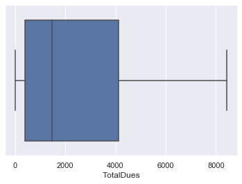
As we can see there is no outlier in this data

Scatter Plot:

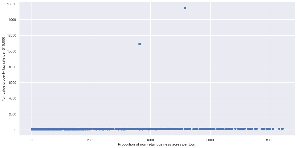
Again checking for outliers, But now we are plotting scatter plot for this. Here we found 3 outliersin total dues. We again removed it by taking mean of the available values There are certainlyother ways too, but this works best for our problem.

Removing Outlier:

Here we are removing the outlier by simply providing the threshold value. The values above thatthreshold will be removed. And values below that threshold will be kept in our dataframe and later those values will be used as an input to our dataframe.

	gender	Management	USAcitizen	Married	MonthsInUnion	ContinuingEd	PaperlessBilling	MonthlyDues	TotalDues	LeftUnion	...	conn_Dial-in	conn_Fiber optic	conn_other	dues_F_Month-to-month	dues_F_One year	dues_F_Two year	pay_M_Bank transfer (automatic)	pay_M_Credit card (automatic)	pay_M_Electronic check	pay_M_Mailed check
0	1	0	1	1	2	1	0	70	144.0	No	...	0	1	0	1	0	0	0	0	0	1
1	0	0	0	0	16	1	1	54	834.0	Yes	...	0	0	0	1	0	0	0	0	0	1
2	1	1	0	0	7	1	0	74	545.0	Yes	...	0	1	0	1	0	0	0	0	0	1
3	1	0	0	0	26	1	1	86	2147.0	No	...	0	1	0	1	0	0	0	0	1	0
4	1	0	0	0	2	1	0	45	75.0	Yes	...	0	0	0	1	0	0	0	0	0	1

5 rows × 42 columns

Scatter and violin Plot:

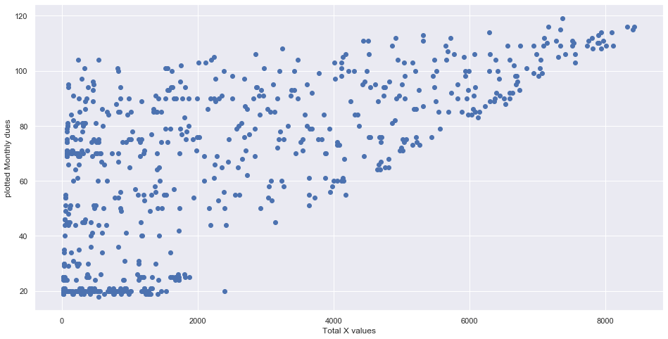
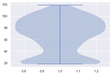
We are again plotting scatter plots to confirm that our outliers has been removed and as we cansee our values are good now. Below we are plotting a Scatter and violin plot. The violin plot simply tells the density about how much distributed values we have in our data.

Scree plot:

Below we are plotting the scree plot for monthly dues column to see how are distributed our values. It’s another way of visualization. We are using matplotlib library for scree plot.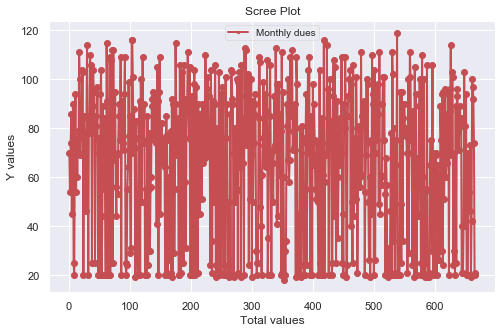

Bivariate plot:

Below we are plotting a Bivariate plot between monthly dues and Months in union to see the difference between both the column values.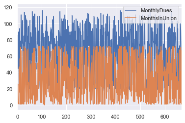

Normalization

After plotting we are normalizing our columns. Normalization simply convert values between 0 and 1.

	MonthsInUnion	MonthlyDues	TotalDues
0	2	70	144.0
1	16	54	834.0
2	7	74	545.0
3	26	86	2147.0
4	2	45	75.0

sc = StandardScaler()
df_train_new_num = sc.fit_transform(df_train_new_num)
(np.mean(df_train_new_num), np.std(df_train_new_num))

(7.1125398974985e-18, 1.0)

	gender	Management	USAcitizen	Married	ContinuingEd	PaperlessBilling	LeftUnion	A_Maryville	A_No	A_Yes	...	conn_Dial-in	conn_Fiber optic	conn_other	dues_F_Month-to-month	dues_F_One year	dues_F_Two year	pay_M_Bank transfer (automatic)	pay_M_Credit card (automatic)	pay_M_Electronic check	pay_M_Mailed check
0	1	0	1	1	1	0	No	0	1	0	...	0	1	0	1	0	0	0	0	0	1
1	0	0	0	0	1	1	Yes	0	1	0	...	0	0	0	1	0	0	0	0	0	1
2	1	1	0	0	1	0	Yes	0	0	1	...	0	1	0	1	0	0	0	0	0	1
3	1	0	0	0	1	1	No	0	1	0	...	0	1	0	1	0	0	0	0	1	0
4	1	0	0	0	1	0	Yes	0	1	0	...	0	0	0	1	0	0	0	0	0	1

5 rows × 39 columns

	MonthsInUnion	MonthlyDues	TotalDues
0	-1.246752	0.151339	-0.960675
1	-0.681128	-0.376021	-0.664369
2	-1.044743	0.283179	-0.788474
3	-0.277110	0.678699	-0.100527
4	-1.246752	-0.672661	-0.990306

	MonthsInUnion	MonthlyDues	TotalDues	gender	Management	USAcitizen	Married	ContinuingEd	PaperlessBilling	LeftUnion	...	conn_Dial-in	conn_Fiber optic	conn_other	dues_F_Month-to-month	dues_F_One year	dues_F_Two year	pay_M_Bank transfer (automatic)	pay_M_Credit card (automatic)	pay_M_Electronic check	pay_M_Mailed check
0	-1.246752	0.151339	-0.960675	1.0	0.0	1.0	1.0	1.0	0.0	No	...	0.0	1.0	0.0	1.0	0.0	0.0	0.0	0.0	0.0	1.0
1	-0.681128	-0.376021	-0.664369	0.0	0.0	0.0	0.0	1.0	1.0	Yes	...	0.0	0.0	0.0	1.0	0.0	0.0	0.0	0.0	0.0	1.0
2	-1.044743	0.283179	-0.788474	1.0	1.0	0.0	0.0	1.0	0.0	Yes	...	0.0	1.0	0.0	1.0	0.0	0.0	0.0	0.0	0.0	1.0
3	-0.277110	0.678699	-0.100527	1.0	0.0	0.0	0.0	1.0	1.0	No	...	0.0	1.0	0.0	1.0	0.0	0.0	0.0	0.0	1.0	0.0
4	-1.246752	-0.672661	-0.990306	1.0	0.0	0.0	0.0	1.0	0.0	Yes	...	0.0	0.0	0.0	1.0	0.0	0.0	0.0	0.0	0.0	1.0

5 rows × 42 columns

	MonthsInUnion	MonthlyDues	TotalDues
0	1	30	30.0
1	34	57	1890.0
2	2	54	108.0
3	45	42	1841.0
4	2	71	152.0

df_test_new_num = sc.fit_transform(df_test_new_num)
(np.mean(df_test_new_num), np.std(df_test_new_num))

(6.963318810448982e-17, 1.0)

df_test_new_cat = df_test_new.drop(['MonthsInUnion','MonthlyDues','TotalDues'] , axis = 1)
df_test_new_cat.head()

	gender	Management	USAcitizen	Married	ContinuingEd	PaperlessBilling	A_Maryville	A_No	A_Yes	B_Maryville	...	conn_Dial-in	conn_Fiber optic	conn_other	dues_F_Month-to-month	dues_F_One year	dues_F_Two year	pay_M_Bank transfer (automatic)	pay_M_Credit card (automatic)	pay_M_Electronic check	pay_M_Mailed check
0	1	0	1	0	0	1	1	0	0	0	...	0	0	0	1	0	0	0	0	1	0
1	0	0	0	0	1	0	0	1	0	0	...	0	0	0	0	1	0	0	0	0	1
2	0	0	0	0	1	1	0	1	0	0	...	0	0	0	1	0	0	0	0	0	1
3	0	0	0	0	0	0	1	0	0	0	...	0	0	0	0	1	0	1	0	0	0
4	1	0	0	0	1	1	0	1	0	0	...	0	1	0	1	0	0	0	0	1	0

5 rows × 38 columns

df_test_new_num = pd.DataFrame(df_test_new_num, columns = ['MonthsInUnion','MonthlyDues','TotalDues'])  
df_test_new_num.head()

	MonthsInUnion	MonthlyDues	TotalDues
0	-1.268931	-1.154574	-0.990430
1	0.070734	-0.258882	-0.169917
2	-1.228335	-0.358403	-0.956021
3	0.517289	-0.756488	-0.191533
4	-1.228335	0.205551	-0.936611

df_test_final = pd.concat([df_test_new_num, df_test_new_cat], axis = 1)
df_test_final.head()

	MonthsInUnion	MonthlyDues	TotalDues	gender	Management	USAcitizen	Married	ContinuingEd	PaperlessBilling	A_Maryville	...	conn_Dial-in	conn_Fiber optic	conn_other	dues_F_Month-to-month	dues_F_One year	dues_F_Two year	pay_M_Bank transfer (automatic)	pay_M_Credit card (automatic)	pay_M_Electronic check	pay_M_Mailed check
0	-1.268931	-1.154574	-0.990430	1	0	1	0	0	1	1	...	0	0	0	1	0	0	0	0	1	0
1	0.070734	-0.258882	-0.169917	0	0	0	0	1	0	0	...	0	0	0	0	1	0	0	0	0	1
2	-1.228335	-0.358403	-0.956021	0	0	0	0	1	1	0	...	0	0	0	1	0	0	0	0	0	1
3	0.517289	-0.756488	-0.191533	0	0	0	0	0	0	1	...	0	0	0	0	1	0	1	0	0	0
4	-1.228335	0.205551	-0.936611	1	0	0	0	1	1	0	...	0	1	0	1	0	0	0	0	1	0

5 rows × 41 columns

Perform a PCA

Train and Test Split:

Here we are separating train test data along with their labels. So that we can perform training. We are using the drop keyword in order to drop the label column from our dataframe. Same process goes with the train and test dataframe.

X_train = df_train_final.drop(['LeftUnion'], axis = 1)
y_train = df_train_final['LeftUnion']
componentsWanted = len(X_train.columns)
print(f'Components wanted = {componentsWanted}')
componentList = ['component'+ str(n) for n in range(componentsWanted)]

Components wanted = 41

X_train.isnull().sum()

MonthsInUnion                      3
MonthlyDues                        3
TotalDues                          3
gender                             3
Management                         3
USAcitizen                         3
Married                            3
ContinuingEd                       3
PaperlessBilling                   3
A_Maryville                        3
A_No                               3
A_Yes                              3
B_Maryville                        3
B_No                               3
B_Yes                              3
C_Maryville                        3
C_No                               3
C_Yes                              3
D_Maryville                        3
D_No                               3
D_Yes                              3
E_Maryville                        3
E_No                               3
E_Yes                              3
F_Maryville                        3
F_No                               3
F_Yes                              3
G_Maryville                        3
G_No                               3
G_Yes                              3
conn_DSL                           3
conn_Dial-in                       3
conn_Fiber optic                   3
conn_other                         3
dues_F_Month-to-month              3
dues_F_One year                    3
dues_F_Two year                    3
pay_M_Bank transfer (automatic)    3
pay_M_Credit card (automatic)      3
pay_M_Electronic check             3
pay_M_Mailed check                 3
dtype: int64

X_train = X_train.dropna()
y_train = y_train.dropna()

pca = PCA(n_components=6)
pca.fit(X_train)
x_pca = pca.transform(X_train)

pca = PCA(n_components=6)
principalComponents_train_data = pca.fit_transform(X_train)
print(principalComponents_train_data.shape)

(663, 6)

principalComponents_train_data_Df = pd.DataFrame(data = principalComponents_train_data, 
                                                 columns = ['p_c_1', 'p_c_2','p_c_3','p_c_4','p_c_5','p_c_6'])
principalComponents_train_data_Df.head()

	p_c_1	p_c_2	p_c_3	p_c_4	p_c_5	p_c_6
0	-1.123156	-1.765350	-0.568427	-0.202989	-0.736615	-0.304088
1	-0.952456	-1.128504	0.248433	0.710367	-1.043984	-0.181601
2	-0.733406	-1.910995	-0.745070	-0.098707	-0.033341	-0.329689
3	0.376765	-1.248122	-1.049732	-0.300304	-0.040315	-0.259779
4	-1.725237	-1.782674	-0.129725	0.761185	-0.857132	0.426444

X_train.head()

	MonthsInUnion	MonthlyDues	TotalDues	gender	Management	USAcitizen	Married	ContinuingEd	PaperlessBilling	A_Maryville	...	conn_Dial-in	conn_Fiber optic	conn_other	dues_F_Month-to-month	dues_F_One year	dues_F_Two year	pay_M_Bank transfer (automatic)	pay_M_Credit card (automatic)	pay_M_Electronic check	pay_M_Mailed check
0	-1.246752	0.151339	-0.960675	1.0	0.0	1.0	1.0	1.0	0.0	0.0	...	0.0	1.0	0.0	1.0	0.0	0.0	0.0	0.0	0.0	1.0
1	-0.681128	-0.376021	-0.664369	0.0	0.0	0.0	0.0	1.0	1.0	0.0	...	0.0	0.0	0.0	1.0	0.0	0.0	0.0	0.0	0.0	1.0
2	-1.044743	0.283179	-0.788474	1.0	1.0	0.0	0.0	1.0	0.0	0.0	...	0.0	1.0	0.0	1.0	0.0	0.0	0.0	0.0	0.0	1.0
3	-0.277110	0.678699	-0.100527	1.0	0.0	0.0	0.0	1.0	1.0	0.0	...	0.0	1.0	0.0	1.0	0.0	0.0	0.0	0.0	1.0	0.0
4	-1.246752	-0.672661	-0.990306	1.0	0.0	0.0	0.0	1.0	0.0	0.0	...	0.0	0.0	0.0	1.0	0.0	0.0	0.0	0.0	0.0	1.0

5 rows × 41 columns

df_comp = pd.DataFrame(pca.components_,index=list(['component 0', 'component 1', 'component 2',
                                                  'component 3','component 4', 'component 5']))
components = df_comp.sort_values(by ='component 0', axis=1,ascending=False).round(decimals=6)
components.transpose()

	component 0	component 1	component 2	component 3	component 4	component 5
2	0.530784	0.251965	-0.227977	0.165887	-0.084599	0.033256
1	0.453539	-0.042664	-0.315131	-0.482817	-0.515765	-0.128799
0	0.430303	0.350500	-0.123795	0.531717	0.242857	0.114482
29	0.160671	-0.015790	0.131636	-0.228592	0.144420	0.285478
14	0.145454	-0.002293	0.195500	-0.222763	0.153149	0.215368
23	0.141642	0.035181	0.268401	-0.107032	0.086999	0.089575
32	0.133672	-0.151133	-0.152434	-0.185538	0.288628	-0.079900
20	0.118569	0.000999	0.199622	0.030107	-0.010979	-0.424902
11	0.112630	-0.011525	0.066390	-0.113220	0.349218	-0.252231
17	0.109808	0.029752	0.269191	0.014545	-0.160624	-0.012298
8	0.102247	-0.103436	-0.022782	-0.102384	0.145836	-0.070760
26	0.094454	0.034455	0.267092	-0.035373	-0.131902	0.174539
5	0.076711	0.065913	0.153082	-0.113436	0.028181	-0.297475
25	0.055811	-0.253331	-0.133304	0.079310	0.126028	-0.142762
16	0.040457	-0.248628	-0.135403	0.029392	0.154749	0.044074
39	0.039411	-0.150297	-0.137597	-0.025898	0.186519	0.005930
19	0.031695	-0.219874	-0.065834	0.013830	0.005104	0.456679
4	0.031681	-0.063952	-0.048477	0.011404	0.097666	-0.004383
36	0.030185	0.145866	0.177738	-0.043666	-0.034665	0.002692
37	0.024472	0.044197	0.088848	-0.004064	-0.011901	-0.051369
38	0.018989	0.063258	0.081571	-0.011789	-0.009277	0.009723
6	0.018854	0.062485	0.113503	-0.043353	-0.064934	-0.148601
30	0.016593	-0.067742	0.286222	0.229476	-0.294502	0.111677
7	0.009757	0.038767	-0.111882	-0.089948	0.095372	-0.033014
22	0.008623	-0.254056	-0.134612	0.150969	-0.092873	-0.057798
35	0.007608	0.085352	0.071200	-0.001251	0.013626	-0.122814
3	0.005905	0.018794	0.026953	0.062345	0.017709	0.020251
13	0.004810	-0.216582	-0.061712	0.266700	-0.159023	-0.183591
9	-0.009757	-0.038767	0.111882	0.089948	-0.095372	0.033014
28	-0.010406	-0.203086	0.002152	0.272529	-0.150294	-0.253701
34	-0.037793	-0.231218	-0.248938	0.044917	0.021039	0.120122
31	-0.047791	0.087520	-0.022428	-0.006308	0.026738	-0.038232
40	-0.082872	0.042842	-0.032823	0.041751	-0.165340	0.035716
33	-0.102474	0.131355	-0.111360	-0.037629	-0.020864	0.006455
10	-0.102873	0.050293	-0.178272	0.023272	-0.253845	0.219217
27	-0.150265	0.218875	-0.133788	-0.043937	0.005874	-0.031777
21	-0.150265	0.218875	-0.133788	-0.043937	0.005874	-0.031777
18	-0.150265	0.218875	-0.133788	-0.043937	0.005874	-0.031777
15	-0.150265	0.218875	-0.133788	-0.043937	0.005874	-0.031777
12	-0.150265	0.218875	-0.133788	-0.043937	0.005874	-0.031777
24	-0.150265	0.218875	-0.133788	-0.043937	0.005874	-0.031777

pca.explained_variance_ratio_

array([0.26047333, 0.16587216, 0.08584148, 0.06586519, 0.05341772,
       0.03435168])

X_train.iloc[:, [12, 15, 18, 21, 24, 27]].head()

	B_Maryville	C_Maryville	D_Maryville	E_Maryville	F_Maryville	G_Maryville
0	0.0	0.0	0.0	0.0	0.0	0.0
1	0.0	0.0	0.0	0.0	0.0	0.0
2	0.0	0.0	0.0	0.0	0.0	0.0
3	0.0	0.0	0.0	0.0	0.0	0.0
4	0.0	0.0	0.0	0.0	0.0	0.0

X_train_final = X_train.drop(['C_Maryville', 'D_Maryville', 'E_Maryville', 'F_Maryville', 'G_Maryville'], axis = 1)
X_train_final.head()

	MonthsInUnion	MonthlyDues	TotalDues	gender	Management	USAcitizen	Married	ContinuingEd	PaperlessBilling	A_Maryville	...	conn_Dial-in	conn_Fiber optic	conn_other	dues_F_Month-to-month	dues_F_One year	dues_F_Two year	pay_M_Bank transfer (automatic)	pay_M_Credit card (automatic)	pay_M_Electronic check	pay_M_Mailed check
0	-1.246752	0.151339	-0.960675	1.0	0.0	1.0	1.0	1.0	0.0	0.0	...	0.0	1.0	0.0	1.0	0.0	0.0	0.0	0.0	0.0	1.0
1	-0.681128	-0.376021	-0.664369	0.0	0.0	0.0	0.0	1.0	1.0	0.0	...	0.0	0.0	0.0	1.0	0.0	0.0	0.0	0.0	0.0	1.0
2	-1.044743	0.283179	-0.788474	1.0	1.0	0.0	0.0	1.0	0.0	0.0	...	0.0	1.0	0.0	1.0	0.0	0.0	0.0	0.0	0.0	1.0
3	-0.277110	0.678699	-0.100527	1.0	0.0	0.0	0.0	1.0	1.0	0.0	...	0.0	1.0	0.0	1.0	0.0	0.0	0.0	0.0	1.0	0.0
4	-1.246752	-0.672661	-0.990306	1.0	0.0	0.0	0.0	1.0	0.0	0.0	...	0.0	0.0	0.0	1.0	0.0	0.0	0.0	0.0	0.0	1.0

5 rows × 36 columns

X_train = df2.drop(['LeftUnion'], axis=1)
table1 = X_train.head()   # Check
# For test set
X_test = df_test.drop(['LeftUnion'], axis=1)
table2 = X_test.head()  # Check
display(table1)
display(table2)

	gender	Management	USAcitizen	Married	MonthsInUnion	ContinuingEd	PaperlessBilling	MonthlyDues	TotalDues	A_Maryville	...	conn_Dial-in	conn_Fiber optic	conn_other	dues_F_Month-to-month	dues_F_One year	dues_F_Two year	pay_M_Bank transfer (automatic)	pay_M_Credit card (automatic)	pay_M_Electronic check	pay_M_Mailed check
0	1	0	1	1	2	1	0	70	144.0	0	...	0	1	0	1	0	0	0	0	0	1
1	0	0	0	0	16	1	1	54	834.0	0	...	0	0	0	1	0	0	0	0	0	1
2	1	1	0	0	7	1	0	74	545.0	0	...	0	1	0	1	0	0	0	0	0	1
3	1	0	0	0	26	1	1	86	2147.0	0	...	0	1	0	1	0	0	0	0	1	0
4	1	0	0	0	2	1	0	45	75.0	0	...	0	0	0	1	0	0	0	0	0	1

5 rows × 41 columns

	gender	Management	USAcitizen	Married	MonthsInUnion	ContinuingEd	PaperlessBilling	MonthlyDues	TotalDues	A_Maryville	...	conn_Dial-in	conn_Fiber optic	conn_other	dues_F_Month-to-month	dues_F_One year	dues_F_Two year	pay_M_Bank transfer (automatic)	pay_M_Credit card (automatic)	pay_M_Electronic check	pay_M_Mailed check
0	1	0	1	0	53	1	0	20	1110	0	...	1	0	0	0	0	1	0	1	0	0
1	1	1	0	0	52	0	1	49	2551	1	...	0	0	0	1	0	0	0	0	1	0
2	0	1	0	0	1	1	0	78	78	0	...	0	1	0	1	0	0	0	0	1	0
3	1	1	0	0	56	1	1	101	5594	0	...	0	1	0	1	0	0	0	0	1	0
4	0	0	0	0	3	1	1	54	140	0	...	0	0	0	1	0	0	0	0	1	0

5 rows × 41 columns

For training set

• Convert series to DataFrame.
• Encoding target values. Encoding target values into 1 and 0.

y_train = df2["LeftUnion"]
y_train = y_train.to_frame()
table1 = y_train.head()
y_train = y_train.astype(str).apply(encode)
table2 = y_train.head()
display(table1)
display(table2)

	LeftUnion
0	No
1	Yes
2	Yes
3	No
4	Yes

	LeftUnion
0	0
1	1
2	1
3	0
4	1

For testing set

• Convert series to df.
• Encoding target values. Encoding target values into 1 and 0.

y_test = df_test["LeftUnion"]
y_test = y_test.to_frame()
table1 = y_test.head()
y_test = y_test.apply(encode)
table2 = y_test.head()
display(table1)
display(table2)

	LeftUnion
0	No
1	Yes
2	Yes
3	No
4	No

	LeftUnion
0	0
1	1
2	1
3	0
4	0

Fitting models

Regression model

In this model we achieved fairly high accuracy.

logisticRegr = LogisticRegression(solver='lbfgs',max_iter=1000)
logisticRegr.fit(X_train.values, y_train.values.ravel())

LogisticRegression(C=1.0, class_weight=None, dual=False, fit_intercept=True,
                   intercept_scaling=1, l1_ratio=None, max_iter=1000,
                   multi_class='auto', n_jobs=None, penalty='l2',
                   random_state=None, solver='lbfgs', tol=0.0001, verbose=0,
                   warm_start=False)

y_pred = logisticRegr.predict(X_test)
print(y_pred)

[0 0 1 0 1 0 0 0 0 0 0 0 0 0 0 0 0 1 0 0 0 0 1 1 0 0 0 0 1 0 0 1 1 0 1 0 1
 1 1 0 0 0 1 0 1 1 0 0 1 0 1 0 0 0 0 0 0 0 0 0 1 0 0 0 0 0 0 0 1 0 0 0 1 0
 0 0 0 0 1 0 0 0 0 0 0 0 1 0 0 0 0 0 0 1 0 0 0 0 0 0 1 0 0 0 0 0 0 1 0 0 0
 1 0 0 1 0 1 0 0 0 0 1 0 1 1 1 0 0 1 0 1 0 0 1 0 0 1 1 1 0 0 0 1 1 0 0 0 0
 0 0 1 0 1 0 0 0 1 0 0 1 0 0 0 0 0 0 1 0 1 0 0 1 0 1 0 1 0 0 0 0 0 0 0 0 0
 0 1 1 0 0 0 0 1 0 0 0 1 0 1 0 0 0 1 0 0 1 0 1 0 0 0 0 1 1 0 0 0 0 0 0 0 0
 0 0 0 1 0 0 1 0 0 0 0 0 0 0 1 0 0 0 0 0 1 0 0 0 0 0 0 0 0 1 0 0 1 0 0 0 1
 0 0 0 1 1 1 0 0 0 0 1 0 0 0 0 0 0 0 0 1 0 1 1 0 1 0 0 0 1 0 0 0 0 0 1 1 0
 0 0 1 0 0 0 0 1 0 0 0 0 0 0 1 0 0 0 1 1 1 0 0 0 0 1 0 0 0 0 0 0 0 0]

Plot Confusion Matrix

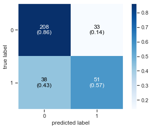
Printing the Accuracy Score

Accuracy Score : 0.78

Diplay Classification report as Data Frame

	precision	recall	f1-score	support
0	0.845528	0.863071	0.854209	241.000000
1	0.607143	0.573034	0.589595	89.000000
accuracy	0.784848	0.784848	0.784848	0.784848
macro avg	0.726336	0.718052	0.721902	330.000000
weighted avg	0.781237	0.784848	0.782844	330.000000

Testing with new dataset

pred = logisticRegr.predict(test_set[0:100])
print(pred)

[1 0 0 0 1 1 0 0 1 0 0 0 0 0 1 0 0 0 0 1 1 0 0 0 0 0 0 0 0 0 0 1 0 0 1 0 1
 0 0 1 0 0 0 0 0 0 0 1 0 0 0 0 0 1 0 1 0 0 0 0 0 0 0 0 1 0 0 0 0 0 0 0 0 0
 1 0 0 0 0 0 1 0 1 0 0 1 0 0 0 0 0 1 0 0 0 1 0 0 0 1]

Decision tree model

[0 0 1 0 1 0 0 0 0 0 1 0 0 1 0 1 0 1 0 0 0 0 1 0 0 0 0 0 1 0 0 1 1 0 1 0 1
 1 1 0 0 0 0 0 1 1 1 0 0 0 0 0 0 0 0 0 0 0 0 0 1 0 0 0 0 0 0 1 0 0 1 1 1 0
 1 0 1 0 0 1 1 0 1 0 0 0 0 0 0 0 0 0 0 1 0 1 0 1 0 0 1 0 0 0 0 0 0 0 0 0 0
 1 0 0 1 0 1 1 0 0 0 0 0 1 0 0 0 0 1 0 1 0 1 1 0 1 0 0 0 1 1 0 1 0 0 0 0 0
 0 0 1 1 1 0 0 1 1 0 0 0 1 0 0 1 0 0 0 0 1 1 0 1 0 1 0 0 0 0 0 0 0 0 0 0 0
 0 0 1 0 0 1 0 1 0 0 0 1 0 1 0 0 0 1 0 0 0 0 1 0 1 0 0 1 1 1 0 0 0 0 0 0 0
 0 1 0 1 0 0 0 0 0 0 0 0 0 0 0 0 0 0 0 1 1 0 0 0 0 0 0 1 0 0 0 0 0 0 0 0 0
 0 0 0 1 1 0 0 1 0 1 1 0 0 1 1 0 0 0 0 1 0 1 1 0 0 1 0 0 0 0 0 0 0 1 1 1 0
 0 0 0 0 0 0 0 1 0 0 0 0 0 0 0 0 0 1 0 0 1 0 0 0 1 1 0 0 0 0 0 0 0 0]

Plot Confusion Matrix

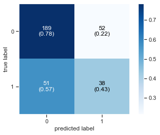
Printing the Accuracy Score

Accuracy Score : 0.69

Diplay Classification report as Data Frame

	precision	recall	f1-score	support
0	0.787500	0.784232	0.785863	241.000000
1	0.422222	0.426966	0.424581	89.000000
accuracy	0.687879	0.687879	0.687879	0.687879
macro avg	0.604861	0.605599	0.605222	330.000000
weighted avg	0.688986	0.687879	0.688426	330.000000

Support Vector Machine

Now here we are running our support vector machine model and we got fairly good accuracy ontest set

[0 0 0 0 0 0 0 0 0 0 0 0 0 0 0 0 0 0 0 0 0 0 0 0 0 0 0 0 0 0 0 0 0 0 0 0 0
 0 0 0 0 0 0 0 0 0 0 0 0 0 0 0 0 0 0 0 0 0 0 0 0 0 0 0 0 0 0 0 0 0 0 0 0 0
 0 0 0 0 0 0 0 0 0 0 0 0 0 0 0 0 0 0 0 0 0 0 0 0 0 0 0 0 0 0 0 0 0 0 0 0 0
 0 0 0 0 0 0 0 0 0 0 0 0 0 0 0 0 0 0 0 0 0 0 0 0 0 0 0 0 0 0 0 0 0 0 0 0 0
 0 0 0 0 0 0 0 0 0 0 0 0 0 0 0 0 0 0 0 0 0 0 0 0 0 0 0 0 0 0 0 0 0 0 0 0 0
 0 0 0 0 0 0 0 0 0 0 0 0 0 0 0 0 0 0 0 0 0 0 0 0 0 0 0 0 0 0 0 0 0 0 0 0 0
 0 0 0 0 0 0 0 0 0 0 0 0 0 0 0 0 0 0 0 0 0 0 0 0 0 0 0 0 0 0 0 0 0 0 0 0 0
 0 0 0 0 0 0 0 0 0 0 0 0 0 0 0 0 0 0 0 0 0 0 0 0 0 0 0 0 0 0 0 0 0 0 0 0 0
 0 0 0 0 0 0 0 0 0 0 0 0 0 0 0 0 0 0 0 0 0 0 0 0 0 0 0 0 0 0 0 0 0 0]

Plot Confusion Matrix

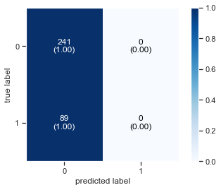
Printing the Accuracy Score

Accuracy Score : 0.73

Diplay Classification report as Data Frame

	precision	recall	f1-score	support
0	0.730303	1.000000	0.844133	241.000000
1	0.000000	0.000000	0.000000	89.000000
accuracy	0.730303	0.730303	0.730303	0.730303
macro avg	0.365152	0.500000	0.422067	330.000000
weighted avg	0.533343	0.730303	0.616473	330.000000

Random Forest

Time to play with a random forest model. It’s an ensemble technique which utilized multiple trees in order to learn best features and perform well on test set. It’s a very famous machine learning model.

[0 0 1 0 0 0 0 0 0 0 0 0 0 0 0 0 0 1 0 0 0 0 1 0 0 0 0 0 1 0 0 1 1 0 1 1 1
 1 0 0 0 0 0 0 1 0 0 0 1 0 1 0 0 0 0 0 0 0 0 0 0 0 0 0 0 0 0 0 0 0 1 0 1 0
 1 0 0 0 0 0 0 0 1 0 0 0 1 0 0 0 0 0 0 1 0 0 1 0 0 0 1 0 0 0 0 0 0 0 0 0 0
 1 0 0 0 0 0 0 0 0 0 1 0 1 1 1 0 0 1 0 1 0 0 1 0 0 1 0 1 0 0 0 1 1 0 0 0 0
 0 0 1 0 1 0 0 0 1 0 0 1 0 0 0 0 0 0 0 0 1 1 0 1 0 1 0 0 0 0 0 0 0 0 1 0 0
 0 1 1 0 0 0 0 1 0 0 0 1 0 1 0 0 0 1 0 0 1 0 1 0 0 0 0 1 0 0 0 0 0 0 0 0 0
 0 0 0 1 0 0 1 0 0 0 0 0 0 0 1 0 0 0 0 0 1 0 0 0 0 0 0 0 0 1 0 0 1 0 0 0 0
 0 0 0 0 0 1 0 0 0 0 1 0 0 0 0 0 0 0 0 1 0 1 1 0 1 1 0 0 1 0 0 0 0 0 1 1 0
 0 0 0 0 0 0 0 0 0 0 0 0 0 0 1 0 0 0 0 1 1 0 0 0 0 1 0 0 0 0 0 0 0 0]

Plot Confusion Matrix

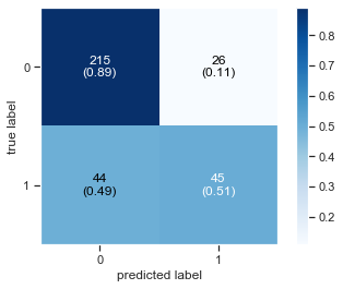
Printing the Accuracy Score

Accuracy Score : 0.79

Diplay Classification report as Data Frame

	precision	recall	f1-score	support
0	0.830116	0.892116	0.860000	241.000000
1	0.633803	0.505618	0.562500	89.000000
accuracy	0.787879	0.787879	0.787879	0.787879
macro avg	0.731959	0.698867	0.711250	330.000000
weighted avg	0.777171	0.787879	0.779765	330.000000

Neural Network

Now we trained a neural network to see how well our model is performing on a simple DNNnetwork.

WARNING:tensorflow:From /opt/anaconda3/envs/tensorflow/lib/python3.6/site-packages/tensorflow/python/ops/init_ops.py:1251: calling VarianceScaling.__init__ (from tensorflow.python.ops.init_ops) with dtype is deprecated and will be removed in a future version.
Instructions for updating:
Call initializer instance with the dtype argument instead of passing it to the constructor
Model: "sequential"
_________________________________________________________________
Layer (type)                 Output Shape              Param #   
=================================================================
dense (Dense)                (None, 12)                504       
_________________________________________________________________
dense_1 (Dense)              (None, 8)                 104       
_________________________________________________________________
dense_2 (Dense)              (None, 1)                 9         
=================================================================
Total params: 617
Trainable params: 617
Non-trainable params: 0
_________________________________________________________________

Compile and fit the keras model

WARNING:tensorflow:From /opt/anaconda3/envs/tensorflow/lib/python3.6/site-packages/tensorflow/python/ops/nn_impl.py:180: add_dispatch_support.<locals>.wrapper (from tensorflow.python.ops.array_ops) is deprecated and will be removed in a future version.
Instructions for updating:
Use tf.where in 2.0, which has the same broadcast rule as np.where
Epoch 1/150
666/666 [==============================] - 0s 362us/sample - loss: 8.2351 - acc: 0.7402
Epoch 2/150
666/666 [==============================] - 0s 152us/sample - loss: 0.7725 - acc: 0.6877
Epoch 3/150
666/666 [==============================] - 0s 146us/sample - loss: 0.5178 - acc: 0.7387
Epoch 4/150
666/666 [==============================] - 0s 148us/sample - loss: 0.5769 - acc: 0.7462
Epoch 5/150
666/666 [==============================] - 0s 163us/sample - loss: 0.6633 - acc: 0.7342
Epoch 6/150
666/666 [==============================] - 0s 148us/sample - loss: 0.5178 - acc: 0.7553
Epoch 7/150
666/666 [==============================] - 0s 149us/sample - loss: 0.5436 - acc: 0.7598
Epoch 8/150
666/666 [==============================] - 0s 149us/sample - loss: 0.5062 - acc: 0.7838
Epoch 9/150
666/666 [==============================] - 0s 145us/sample - loss: 0.5271 - acc: 0.7853
Epoch 10/150
666/666 [==============================] - 0s 149us/sample - loss: 0.4971 - acc: 0.7748
Epoch 11/150
666/666 [==============================] - 0s 145us/sample - loss: 0.4631 - acc: 0.7973
Epoch 12/150
666/666 [==============================] - 0s 146us/sample - loss: 0.6097 - acc: 0.7538
Epoch 13/150
666/666 [==============================] - 0s 147us/sample - loss: 0.4964 - acc: 0.7838
Epoch 14/150
666/666 [==============================] - 0s 145us/sample - loss: 0.4721 - acc: 0.7748
Epoch 15/150
666/666 [==============================] - 0s 151us/sample - loss: 0.4736 - acc: 0.7853
Epoch 16/150
666/666 [==============================] - 0s 142us/sample - loss: 0.5045 - acc: 0.8018
Epoch 17/150
666/666 [==============================] - 0s 141us/sample - loss: 0.5331 - acc: 0.7838
Epoch 18/150
666/666 [==============================] - 0s 141us/sample - loss: 0.5281 - acc: 0.7823
Epoch 19/150
666/666 [==============================] - 0s 145us/sample - loss: 0.4544 - acc: 0.8018
Epoch 20/150
666/666 [==============================] - 0s 146us/sample - loss: 0.4513 - acc: 0.8063
Epoch 21/150
666/666 [==============================] - 0s 146us/sample - loss: 0.4966 - acc: 0.7883
Epoch 22/150
666/666 [==============================] - 0s 152us/sample - loss: 0.5678 - acc: 0.7763
Epoch 23/150
666/666 [==============================] - 0s 148us/sample - loss: 0.4587 - acc: 0.8123
Epoch 24/150
666/666 [==============================] - 0s 146us/sample - loss: 0.4463 - acc: 0.8003
Epoch 25/150
666/666 [==============================] - 0s 153us/sample - loss: 0.4676 - acc: 0.7988
Epoch 26/150
666/666 [==============================] - 0s 146us/sample - loss: 0.4695 - acc: 0.8003
Epoch 27/150
666/666 [==============================] - 0s 141us/sample - loss: 0.5317 - acc: 0.7868
Epoch 28/150
666/666 [==============================] - 0s 143us/sample - loss: 0.4589 - acc: 0.8033
Epoch 29/150
666/666 [==============================] - 0s 145us/sample - loss: 0.4937 - acc: 0.7913
Epoch 30/150
666/666 [==============================] - 0s 146us/sample - loss: 0.4410 - acc: 0.8018
Epoch 31/150
666/666 [==============================] - 0s 147us/sample - loss: 0.4422 - acc: 0.8078
Epoch 32/150
666/666 [==============================] - 0s 147us/sample - loss: 0.4714 - acc: 0.8093
Epoch 33/150
666/666 [==============================] - 0s 149us/sample - loss: 0.4257 - acc: 0.8093
Epoch 34/150
666/666 [==============================] - 0s 150us/sample - loss: 0.4649 - acc: 0.8018
Epoch 35/150
666/666 [==============================] - 0s 147us/sample - loss: 0.4341 - acc: 0.8123
Epoch 36/150
666/666 [==============================] - 0s 140us/sample - loss: 0.4822 - acc: 0.7868
Epoch 37/150
666/666 [==============================] - 0s 143us/sample - loss: 0.4445 - acc: 0.7988
Epoch 38/150
666/666 [==============================] - 0s 144us/sample - loss: 0.4484 - acc: 0.8078
Epoch 39/150
666/666 [==============================] - 0s 161us/sample - loss: 0.4193 - acc: 0.8138
Epoch 40/150
666/666 [==============================] - 0s 154us/sample - loss: 0.4386 - acc: 0.8108
Epoch 41/150
666/666 [==============================] - 0s 144us/sample - loss: 0.4781 - acc: 0.7808
Epoch 42/150
666/666 [==============================] - 0s 143us/sample - loss: 0.4706 - acc: 0.7868
Epoch 43/150
666/666 [==============================] - 0s 142us/sample - loss: 0.4562 - acc: 0.8078
Epoch 44/150
666/666 [==============================] - 0s 142us/sample - loss: 0.5031 - acc: 0.7958
Epoch 45/150
666/666 [==============================] - 0s 144us/sample - loss: 0.4337 - acc: 0.8108
Epoch 46/150
666/666 [==============================] - 0s 150us/sample - loss: 0.4187 - acc: 0.8093
Epoch 47/150
666/666 [==============================] - 0s 136us/sample - loss: 0.4294 - acc: 0.8183
Epoch 48/150
666/666 [==============================] - 0s 139us/sample - loss: 0.4279 - acc: 0.8063
Epoch 49/150
666/666 [==============================] - 0s 138us/sample - loss: 0.4331 - acc: 0.8078
Epoch 50/150
666/666 [==============================] - 0s 139us/sample - loss: 0.4395 - acc: 0.8168
Epoch 51/150
666/666 [==============================] - 0s 139us/sample - loss: 0.4346 - acc: 0.8018
Epoch 52/150
666/666 [==============================] - 0s 139us/sample - loss: 0.4352 - acc: 0.8138
Epoch 53/150
666/666 [==============================] - 0s 139us/sample - loss: 0.4642 - acc: 0.8063
Epoch 54/150
666/666 [==============================] - 0s 140us/sample - loss: 0.4376 - acc: 0.8153
Epoch 55/150
666/666 [==============================] - 0s 141us/sample - loss: 0.4242 - acc: 0.8153
Epoch 56/150
666/666 [==============================] - 0s 146us/sample - loss: 0.4332 - acc: 0.8153
Epoch 57/150
666/666 [==============================] - 0s 143us/sample - loss: 0.4424 - acc: 0.8183
Epoch 58/150
666/666 [==============================] - 0s 143us/sample - loss: 0.4302 - acc: 0.8033
Epoch 59/150
666/666 [==============================] - 0s 141us/sample - loss: 0.4294 - acc: 0.8093
Epoch 60/150
666/666 [==============================] - 0s 144us/sample - loss: 0.4540 - acc: 0.8048
Epoch 61/150
666/666 [==============================] - 0s 140us/sample - loss: 0.4212 - acc: 0.8168
Epoch 62/150
666/666 [==============================] - 0s 138us/sample - loss: 0.4194 - acc: 0.8138
Epoch 63/150
666/666 [==============================] - 0s 137us/sample - loss: 0.4234 - acc: 0.8228
Epoch 64/150
666/666 [==============================] - 0s 140us/sample - loss: 0.4249 - acc: 0.8213
Epoch 65/150
666/666 [==============================] - 0s 139us/sample - loss: 0.4191 - acc: 0.8138
Epoch 66/150
666/666 [==============================] - 0s 143us/sample - loss: 0.4366 - acc: 0.8108
Epoch 67/150
666/666 [==============================] - 0s 143us/sample - loss: 0.4382 - acc: 0.8228
Epoch 68/150
666/666 [==============================] - 0s 144us/sample - loss: 0.4391 - acc: 0.8078
Epoch 69/150
666/666 [==============================] - 0s 144us/sample - loss: 0.4370 - acc: 0.8108
Epoch 70/150
666/666 [==============================] - 0s 143us/sample - loss: 0.4195 - acc: 0.8198
Epoch 71/150
666/666 [==============================] - 0s 144us/sample - loss: 0.4275 - acc: 0.8228
Epoch 72/150
666/666 [==============================] - 0s 141us/sample - loss: 0.4212 - acc: 0.8153
Epoch 73/150
666/666 [==============================] - 0s 139us/sample - loss: 0.4196 - acc: 0.8258
Epoch 74/150
666/666 [==============================] - 0s 140us/sample - loss: 0.4067 - acc: 0.8198
Epoch 75/150
666/666 [==============================] - 0s 139us/sample - loss: 0.4134 - acc: 0.8108
Epoch 76/150
666/666 [==============================] - 0s 143us/sample - loss: 0.4258 - acc: 0.8048
Epoch 77/150
666/666 [==============================] - 0s 141us/sample - loss: 0.4170 - acc: 0.8243
Epoch 78/150
666/666 [==============================] - 0s 141us/sample - loss: 0.4303 - acc: 0.8138
Epoch 79/150
666/666 [==============================] - 0s 140us/sample - loss: 0.4320 - acc: 0.8138
Epoch 80/150
666/666 [==============================] - 0s 137us/sample - loss: 0.4277 - acc: 0.8258
Epoch 81/150
666/666 [==============================] - 0s 139us/sample - loss: 0.3979 - acc: 0.8288
Epoch 82/150
666/666 [==============================] - 0s 141us/sample - loss: 0.4183 - acc: 0.8303
Epoch 83/150
666/666 [==============================] - 0s 149us/sample - loss: 0.4195 - acc: 0.8108
Epoch 84/150
666/666 [==============================] - 0s 149us/sample - loss: 0.4228 - acc: 0.8243
Epoch 85/150
666/666 [==============================] - 0s 146us/sample - loss: 0.4082 - acc: 0.8288
Epoch 86/150
666/666 [==============================] - 0s 154us/sample - loss: 0.4287 - acc: 0.8108
Epoch 87/150
666/666 [==============================] - 0s 138us/sample - loss: 0.4302 - acc: 0.8213
Epoch 88/150
666/666 [==============================] - 0s 138us/sample - loss: 0.4091 - acc: 0.8138
Epoch 89/150
666/666 [==============================] - 0s 137us/sample - loss: 0.4217 - acc: 0.8288
Epoch 90/150
666/666 [==============================] - 0s 138us/sample - loss: 0.4184 - acc: 0.8213
Epoch 91/150
666/666 [==============================] - 0s 140us/sample - loss: 0.4188 - acc: 0.8408
Epoch 92/150
666/666 [==============================] - 0s 138us/sample - loss: 0.4051 - acc: 0.8333
Epoch 93/150
666/666 [==============================] - 0s 137us/sample - loss: 0.4059 - acc: 0.8258
Epoch 94/150
666/666 [==============================] - 0s 138us/sample - loss: 0.4019 - acc: 0.8273
Epoch 95/150
666/666 [==============================] - 0s 137us/sample - loss: 0.4329 - acc: 0.8108
Epoch 96/150
666/666 [==============================] - 0s 138us/sample - loss: 0.4018 - acc: 0.8393
Epoch 97/150
666/666 [==============================] - 0s 146us/sample - loss: 0.4083 - acc: 0.8348
Epoch 98/150
666/666 [==============================] - 0s 142us/sample - loss: 0.4087 - acc: 0.8243
Epoch 99/150
666/666 [==============================] - 0s 142us/sample - loss: 0.4468 - acc: 0.8228
Epoch 100/150
666/666 [==============================] - 0s 138us/sample - loss: 0.4129 - acc: 0.8198
Epoch 101/150
666/666 [==============================] - 0s 137us/sample - loss: 0.4327 - acc: 0.8258
Epoch 102/150
666/666 [==============================] - 0s 138us/sample - loss: 0.4063 - acc: 0.8318
Epoch 103/150
666/666 [==============================] - 0s 138us/sample - loss: 0.4068 - acc: 0.8318
Epoch 104/150
666/666 [==============================] - 0s 140us/sample - loss: 0.4083 - acc: 0.8303
Epoch 105/150
666/666 [==============================] - 0s 143us/sample - loss: 0.3960 - acc: 0.8213
Epoch 106/150
666/666 [==============================] - 0s 140us/sample - loss: 0.4094 - acc: 0.8258
Epoch 107/150
666/666 [==============================] - 0s 144us/sample - loss: 0.4313 - acc: 0.8243
Epoch 108/150
666/666 [==============================] - 0s 138us/sample - loss: 0.4163 - acc: 0.8363
Epoch 109/150
666/666 [==============================] - 0s 139us/sample - loss: 0.4072 - acc: 0.8273
Epoch 110/150
666/666 [==============================] - 0s 138us/sample - loss: 0.4113 - acc: 0.8183
Epoch 111/150
666/666 [==============================] - 0s 137us/sample - loss: 0.3955 - acc: 0.8378
Epoch 112/150
666/666 [==============================] - 0s 138us/sample - loss: 0.4096 - acc: 0.8408
Epoch 113/150
666/666 [==============================] - 0s 139us/sample - loss: 0.4099 - acc: 0.8348
Epoch 114/150
666/666 [==============================] - 0s 140us/sample - loss: 0.4026 - acc: 0.8198
Epoch 115/150
666/666 [==============================] - 0s 139us/sample - loss: 0.3947 - acc: 0.8333
Epoch 116/150
666/666 [==============================] - 0s 140us/sample - loss: 0.4073 - acc: 0.8333
Epoch 117/150
666/666 [==============================] - 0s 137us/sample - loss: 0.4155 - acc: 0.8243
Epoch 118/150
666/666 [==============================] - 0s 142us/sample - loss: 0.4025 - acc: 0.8378
Epoch 119/150
666/666 [==============================] - 0s 140us/sample - loss: 0.3951 - acc: 0.8333
Epoch 120/150
666/666 [==============================] - 0s 143us/sample - loss: 0.3934 - acc: 0.8333
Epoch 121/150
666/666 [==============================] - 0s 140us/sample - loss: 0.3919 - acc: 0.8348
Epoch 122/150
666/666 [==============================] - 0s 139us/sample - loss: 0.4007 - acc: 0.8318
Epoch 123/150
666/666 [==============================] - 0s 139us/sample - loss: 0.4120 - acc: 0.8153
Epoch 124/150
666/666 [==============================] - 0s 140us/sample - loss: 0.4494 - acc: 0.7883
Epoch 125/150
666/666 [==============================] - 0s 138us/sample - loss: 0.4067 - acc: 0.8108
Epoch 126/150
666/666 [==============================] - 0s 138us/sample - loss: 0.4027 - acc: 0.8048
Epoch 127/150
666/666 [==============================] - 0s 139us/sample - loss: 0.3961 - acc: 0.8408
Epoch 128/150
666/666 [==============================] - 0s 146us/sample - loss: 0.3914 - acc: 0.8333
Epoch 129/150
666/666 [==============================] - 0s 140us/sample - loss: 0.3871 - acc: 0.8498
Epoch 130/150
666/666 [==============================] - 0s 140us/sample - loss: 0.4430 - acc: 0.7868
Epoch 131/150
666/666 [==============================] - 0s 139us/sample - loss: 0.3887 - acc: 0.8378
Epoch 132/150
666/666 [==============================] - 0s 140us/sample - loss: 0.3985 - acc: 0.8243
Epoch 133/150
666/666 [==============================] - 0s 136us/sample - loss: 0.4054 - acc: 0.8213
Epoch 134/150
666/666 [==============================] - 0s 138us/sample - loss: 0.4085 - acc: 0.8243
Epoch 135/150
666/666 [==============================] - 0s 137us/sample - loss: 0.3927 - acc: 0.8333
Epoch 136/150
666/666 [==============================] - 0s 138us/sample - loss: 0.3950 - acc: 0.8333
Epoch 137/150
666/666 [==============================] - 0s 138us/sample - loss: 0.3905 - acc: 0.8348
Epoch 138/150
666/666 [==============================] - 0s 137us/sample - loss: 0.3867 - acc: 0.8438
Epoch 139/150
666/666 [==============================] - 0s 140us/sample - loss: 0.3806 - acc: 0.8348
Epoch 140/150
666/666 [==============================] - 0s 138us/sample - loss: 0.3922 - acc: 0.8348
Epoch 141/150
666/666 [==============================] - 0s 139us/sample - loss: 0.4074 - acc: 0.8153
Epoch 142/150
666/666 [==============================] - 0s 140us/sample - loss: 0.4033 - acc: 0.8303
Epoch 143/150
666/666 [==============================] - 0s 139us/sample - loss: 0.3936 - acc: 0.8228
Epoch 144/150
666/666 [==============================] - 0s 141us/sample - loss: 0.3825 - acc: 0.8468
Epoch 145/150
666/666 [==============================] - 0s 149us/sample - loss: 0.3862 - acc: 0.8258
Epoch 146/150
666/666 [==============================] - 0s 153us/sample - loss: 0.3839 - acc: 0.8423
Epoch 147/150
666/666 [==============================] - 0s 142us/sample - loss: 0.3831 - acc: 0.8363
Epoch 148/150
666/666 [==============================] - 0s 145us/sample - loss: 0.3973 - acc: 0.8243
Epoch 149/150
666/666 [==============================] - 0s 153us/sample - loss: 0.3890 - acc: 0.8423
Epoch 150/150
666/666 [==============================] - 0s 155us/sample - loss: 0.3871 - acc: 0.8438

Evaluate the keras model

666/666 [==============================] - 0s 71us/sample - loss: 0.3759 - acc: 0.8453
Training Accuracy: 84.53
330/330 [==============================] - 0s 30us/sample - loss: 0.4749 - acc: 0.7515
Testing Accuracy: 75.15

Model Prediction

[0 0 1 0 0 0 0 0 0 0 0 0 0 1 0 0 0 1 0 0 0 0 1 0 0 0 0 0 1 0 0 1 1 0 1 0 1
 1 1 0 0 0 1 0 1 1 0 0 1 0 1 0 1 0 0 0 0 0 0 0 1 0 0 0 0 0 0 0 0 0 1 0 1 0
 0 0 0 0 0 0 0 0 1 0 0 1 1 0 0 0 0 0 0 1 0 0 1 0 0 0 1 0 0 0 0 0 0 1 0 0 0
 1 0 0 1 0 1 0 0 0 0 1 0 0 1 1 0 0 1 0 1 0 0 0 0 0 1 1 0 0 0 0 0 1 1 0 0 0
 1 0 1 0 1 0 0 0 0 0 0 0 0 0 0 0 0 0 1 0 1 1 0 1 0 1 0 1 0 0 0 0 0 0 1 0 0
 0 1 1 0 0 0 0 1 1 0 0 1 0 1 0 0 0 1 0 0 1 0 1 0 0 0 0 1 1 1 0 0 0 0 1 0 0
 0 0 0 1 0 0 1 0 1 0 0 0 0 0 1 0 0 0 0 1 1 0 0 0 0 0 0 0 0 1 0 0 1 0 0 0 1
 0 0 0 1 1 1 0 1 0 0 1 0 1 0 0 0 0 0 0 1 0 1 1 0 1 1 0 0 1 1 0 0 0 0 1 1 0
 0 0 1 0 0 0 0 1 0 0 0 0 0 0 1 1 0 0 1 1 1 1 0 0 1 0 0 0 0 0 0 0 0 0]

Plot Confusion Matrix

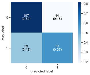
Printing the Accuracy Score

Accuracy Score : 0.75

Diplay Classification report as Data Frame

	precision	recall	f1-score	support
0	0.838298	0.817427	0.827731	241.000000
1	0.536842	0.573034	0.554348	89.000000
accuracy	0.751515	0.751515	0.751515	0.751515
macro avg	0.687570	0.695231	0.691039	330.000000
weighted avg	0.756996	0.751515	0.754000	330.000000

Explain why you think the results differed

In the blind guesses the model is not trained on any kind of data. you just give arandom prediction There is no statistical calculation involved behind the ans. Therefore the results differafter training the model. Because before training the model hasn’t leant anything fromthe data. But after training model has learnt the weights and now can perform better onlearned data.

How you would improve your project if you had more time?

I would apply some advance statistical technique for removing outliers andassigning more weights to the minority classes. Also I would like to do fine tuning byusing pre-trained deep learning model. I would apply more data cleaning techniques toclean out some redundant values.