Predicting Landmark Duration
Photo sharing and photo storage services thrive on location data for the images uploaded by their users. Location data enables useful features like automatic tagging suggestions and organization of photos, greatly enhancing the user experience. However, many uploaded photos lack location metadata due to reasons like cameras lacking GPS or privacy concerns removing metadata.
When no location data is available for an image, one option is to detect and classify any landmarks visible within the image to infer its location. However, the vast number of landmarks worldwide and the enormous volume of uploaded images make manual classification by humans impractical. In this project, we will build models to automatically predict an image’s location based on any landmarks depicted. At the end, our code will accept any user-uploaded image as input and suggest the top k most relevant landmarks from a set of 50 major landmarks globally.
This automated landmark classification approach can compensate for missing location metadata and improve the photos’ discoverability on sharing platforms. The models we develop here represent an initial step, laying the foundation for more advanced models that can detect and classify a wider range of landmarks to determine an image’s precise location.
The Road Ahead
- Step 0: Download Datasets and Install Python Modules
- Step 1: Create a CNN to Classify Landmarks (from Scratch)
- Step 2: Create a CNN to Classify Landmarks (using Transfer Learning)
- Step 3: Write Your Landmark Prediction Algorithm
Step 0: Download Datasets and Install Python Modules
Download the landmark dataset.
Step 1: Create a CNN to Classify Landmarks (from Scratch)
Specify Data Loaders for the Landmark Dataset
Specify appropriate transforms
# # convert data to a normalized torch.FloatTensor
image_transforms = transforms.Compose([transforms.Resize(size=224),
                                       transforms.CenterCrop(size=224),
                                       transforms.RandomRotation(20),
                                       transforms.ToTensor(),
                                       transforms.Normalize([0.485, 0.456, 0.406],
                                                            [0.229, 0.224, 0.225])
                                      ])
Write data loaders for training, validation, and test sets
train_data = datasets.ImageFolder(traindir, transform=image_transforms)
test_data = datasets.ImageFolder(testdir, transform=image_transforms)
loaders_scratch = {'train': torch.utils.data.DataLoader(train_data, batch_size=batch_size,
                                                        sampler=train_sampler, num_workers=num_workers,
                                                       pin_memory=True),
                   'valid': torch.utils.data.DataLoader(train_data, batch_size=batch_size,
                                                        sampler=train_sampler, num_workers=num_workers,
                                                       pin_memory=True),
                   'test': torch.utils.data.DataLoader(test_data, batch_size=batch_size,
                                                       num_workers=num_workers, pin_memory=True)}

# prepare data loaders (combine dataset and sampler)
train_loader = loaders_scratch['train']
valid_loader = loaders_scratch['valid']
test_loader = loaders_scratch['test']

num_classes = len(train_data.classes)
print(num_classes)
50
I resized all image to 224 pixel, center cropped, add randomly rotations for some degrees to avoid overfitting of the model.
I tried to approached the problem iteratively and starting with the examples from this project, I am working with (224, 224, 3) images, so the inputs are significantly bigger than the labs (28, 28, 1) for Mnist and (32x32x3) for CIFAR. I’ve also realized that the most of the pre-trained models require the input to be 224x224 pixel images. Also, I’ll need to match the normalization used when the models were trained. Each color channel has to normalized separately, the means are [0.485, 0.456, 0.406] and the standard deviations are [0.229, 0.224, 0.225].
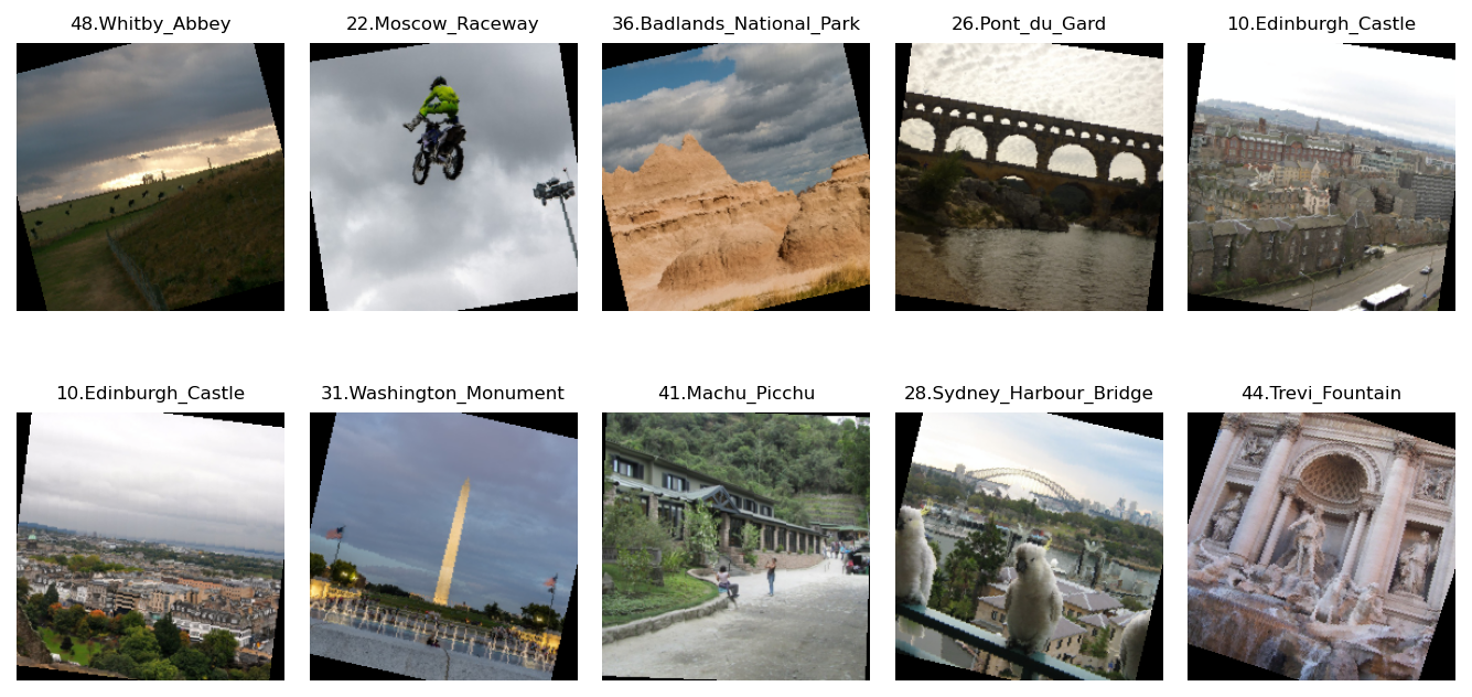
Visualize a Batch of Training Data
Visualizing the output of our data loader.
Specify Loss Function and Optimizer
## TODO: select loss function
criterion_scratch = nn.CrossEntropyLoss()

def get_optimizer_scratch(model):
    ## TODO: select and return an optimizer
    model = optim.AdamW(model.parameters(), lr=0.01)

    return model
Model Architecture
Create a CNN to classify images of landmarks.
create model ... Net(
  (conv1): Conv2d(3, 16, kernel_size=(3, 3), stride=(1, 1), padding=(1, 1))
  (conv2): Conv2d(16, 32, kernel_size=(3, 3), stride=(1, 1), padding=(1, 1))
  (conv3): Conv2d(32, 64, kernel_size=(3, 3), stride=(1, 1), padding=(1, 1))
  (pool): MaxPool2d(kernel_size=2, stride=2, padding=0, dilation=1, ceil_mode=False)
  (fc1): Linear(in_features=50176, out_features=128, bias=True)
  (fc2): Linear(in_features=128, out_features=50, bias=True)
  (dropout): Dropout(p=0.25, inplace=False)
  (batch_norm): BatchNorm1d(128, eps=1e-05, momentum=0.1, affine=True, track_running_stats=True)
)
The first layer in the CNN is a convolutional layer that takes (224, 224, 3) input size of 50 classes.
I’d like the new layer to have 16 filters, each with a height and width of 3. When performing the convolution, I’d like the filter to jump 1 pixel at a time.
_nn.Conv2d(in_channels, out_channels, kernelsize, stride=1, padding=0)
I want this layer to have the same width and height as the input layer, so I will pad accordingly; Then, to construct this convolutional layer, I use the following line of code:
self.conv2 = nn.Conv2d(3, 32, 3, padding=1)
I am adding a pool layer that takes a kernel_size and a stride after every convolution layer. This will down-sample the input’s x-y dimensions, by a factor of 2:
self.pool = nn.MaxPool2d(2,2)
I am adding a fully connected linear layer at the end to produce a 50-dim output. As well as a Dropout layer to avoid overfitting.
A forward pass would give the following structure:
torch.Size([16, 3, 224, 224])

torch.Size([16, 16, 112, 112])

torch.Size([16, 32, 56, 56])

torch.Size([16, 64, 28, 28])

torch.Size([16, 50176])

torch.Size([16, 500])

torch.Size([16, 50])
Experiment with the Weight Initialization
custom weight initialization
def custom_weight_init(m):
    ## TODO: implement a weight initialization strategy
    if isinstance(m, nn.Conv2d):
        m.weight.data.normal_(0, 0.02)
        m.bias.data.zero_()
    elif isinstance(m, nn.Linear):
        m.weight.data.normal_(0, 0.02)
        m.bias.data.zero_()

model_scratch.apply(custom_weight_init)
model_scratch = train(10, loaders_scratch, model_scratch, get_optimizer_scratch(model_scratch),
                      criterion_scratch, use_cuda, 'ignore.pt')
load previous saved model ...
Epoch: 1 	Training Loss: 2.569729 	Validation Loss: 2.100670
Validation loss decreased (inf --> 2.100670).  Saving model ...
Epoch: 2 	Training Loss: 2.365887 	Validation Loss: 2.027413
Validation loss decreased (2.100670 --> 2.027413).  Saving model ...
Epoch: 3 	Training Loss: 2.241768 	Validation Loss: 1.826511
Validation loss decreased (2.027413 --> 1.826511).  Saving model ...
Epoch: 4 	Training Loss: 2.103884 	Validation Loss: 1.659331
Validation loss decreased (1.826511 --> 1.659331).  Saving model ...
Epoch: 5 	Training Loss: 1.985072 	Validation Loss: 1.512019
Validation loss decreased (1.659331 --> 1.512019).  Saving model ...
Epoch: 6 	Training Loss: 1.905725 	Validation Loss: 1.525671
Epoch: 7 	Training Loss: 1.817186 	Validation Loss: 1.337682
Validation loss decreased (1.512019 --> 1.337682).  Saving model ...
Epoch: 8 	Training Loss: 1.722563 	Validation Loss: 1.298211
Validation loss decreased (1.337682 --> 1.298211).  Saving model ...
Epoch: 9 	Training Loss: 1.646949 	Validation Loss: 1.175978
Validation loss decreased (1.298211 --> 1.175978).  Saving model ...
Epoch: 10 	Training Loss: 1.551494 	Validation Loss: 1.034477
Validation loss decreased (1.175978 --> 1.034477).  Saving model ...
Train and Validate the Model
default weight initialization
# reset the model parameters
model_scratch.apply(default_weight_init)

# train the model
model_scratch = train(num_epochs, loaders_scratch, model_scratch, get_optimizer_scratch(model_scratch),
                      criterion_scratch, use_cuda, 'model_scratch.pt')
load previous saved model ...
Epoch: 1 	Training Loss: 2.569074 	Validation Loss: 2.133349
Validation loss decreased (inf --> 2.133349).  Saving model ...
Epoch: 2 	Training Loss: 2.337926 	Validation Loss: 1.954307
Validation loss decreased (2.133349 --> 1.954307).  Saving model ...
Epoch: 3 	Training Loss: 2.189509 	Validation Loss: 1.836033
Validation loss decreased (1.954307 --> 1.836033).  Saving model ...
Epoch: 4 	Training Loss: 2.079099 	Validation Loss: 1.654004
Validation loss decreased (1.836033 --> 1.654004).  Saving model ...
Epoch: 5 	Training Loss: 1.995490 	Validation Loss: 1.567419
Validation loss decreased (1.654004 --> 1.567419).  Saving model ...
Epoch: 6 	Training Loss: 1.863627 	Validation Loss: 1.480632
Validation loss decreased (1.567419 --> 1.480632).  Saving model ...
Epoch: 7 	Training Loss: 1.782091 	Validation Loss: 1.303887
Validation loss decreased (1.480632 --> 1.303887).  Saving model ...
Epoch: 8 	Training Loss: 1.646969 	Validation Loss: 1.191111
Validation loss decreased (1.303887 --> 1.191111).  Saving model ...
Epoch: 9 	Training Loss: 1.545885 	Validation Loss: 1.036899
Validation loss decreased (1.191111 --> 1.036899).  Saving model ...
Epoch: 10 	Training Loss: 1.492636 	Validation Loss: 0.941374
Validation loss decreased (1.036899 --> 0.941374).  Saving model ...
Test the Model
test(loaders_scratch, model_scratch, criterion_scratch, use_cuda)
Test Loss: 3.044593


Test Accuracy: 31% (399/1250)
Step 2: Create a CNN to Classify Landmarks (using Transfer Learning)
We will now use transfer learning to create a CNN that can identify landmarks from images.
Specify Data Loaders for the Landmark Dataset
### TODO: Write data loaders for training, validation, and test sets
## Specify appropriate transforms, and batch_sizes

loaders_transfer = loaders_scratch.copy()
# prepare data loaders (combine dataset and sampler)
train_loader = loaders_transfer['train']
valid_loader = loaders_transfer['valid']
test_loader = loaders_transfer['test']
Specify Loss Function and Optimizer
## TODO: select loss function
criterion_transfer = nn.CrossEntropyLoss()

def get_optimizer_transfer(model):
    ## TODO: select and return optimizer
    model = optim.AdamW(model.parameters(), lr=0.01)
    return model
Model Architecture
Use transfer learning to create a CNN to classify images of landmarks.
## TODO: Specify model architecture
model_transfer =  models.alexnet(pretrained=True)
AlexNet(
  (features): Sequential(
    (0): Conv2d(3, 64, kernel_size=(11, 11), stride=(4, 4), padding=(2, 2))
    (1): ReLU(inplace=True)
    (2): MaxPool2d(kernel_size=3, stride=2, padding=0, dilation=1, ceil_mode=False)
    (3): Conv2d(64, 192, kernel_size=(5, 5), stride=(1, 1), padding=(2, 2))
    (4): ReLU(inplace=True)
    (5): MaxPool2d(kernel_size=3, stride=2, padding=0, dilation=1, ceil_mode=False)
    (6): Conv2d(192, 384, kernel_size=(3, 3), stride=(1, 1), padding=(1, 1))
    (7): ReLU(inplace=True)
    (8): Conv2d(384, 256, kernel_size=(3, 3), stride=(1, 1), padding=(1, 1))
    (9): ReLU(inplace=True)
    (10): Conv2d(256, 256, kernel_size=(3, 3), stride=(1, 1), padding=(1, 1))
    (11): ReLU(inplace=True)
    (12): MaxPool2d(kernel_size=3, stride=2, padding=0, dilation=1, ceil_mode=False)
  )
  (avgpool): AdaptiveAvgPool2d(output_size=(6, 6))
  (classifier): Sequential(
    (0): Dropout(p=0.5, inplace=False)
    (1): Linear(in_features=9216, out_features=4096, bias=True)
    (2): ReLU(inplace=True)
    (3): Dropout(p=0.5, inplace=False)
    (4): Linear(in_features=4096, out_features=4096, bias=True)
    (5): ReLU(inplace=True)
    (6): Linear(in_features=4096, out_features=50, bias=True)
  )
)
I’ll use a alexnet model from torchvision model archiv, which was already trained previously. The classifier part of the model is a single fully-connected layer:
classifier[6]: (6): Linear(in_features=4096, out_features=1000, bias=True)
This layer was already trained on the ImageNet dataset, so it won’t work for the landmark classification specific problem with different output size, means I need to replace the classifier (50 classes).
Train and Validate the Model
Train and validate our model and Save the final model parameters.
model_transfer.load_state_dict(torch.load('model_transfer.pt'))
load previous saved model ...
Epoch: 1 	Training Loss: 4.195210 	Validation Loss: 1.586942
Validation loss decreased (inf --> 1.586942).  Saving model ...
Epoch: 2 	Training Loss: 3.176030 	Validation Loss: 1.186133
Validation loss decreased (1.586942 --> 1.186133).  Saving model ...
Epoch: 3 	Training Loss: 2.868873 	Validation Loss: 1.037404
Validation loss decreased (1.186133 --> 1.037404).  Saving model ...
Epoch: 4 	Training Loss: 2.673997 	Validation Loss: 0.943730
Validation loss decreased (1.037404 --> 0.943730).  Saving model ...
Epoch: 5 	Training Loss: 2.551795 	Validation Loss: 0.916311
Validation loss decreased (0.943730 --> 0.916311).  Saving model ...
Epoch: 6 	Training Loss: 2.399288 	Validation Loss: 0.908761
Validation loss decreased (0.916311 --> 0.908761).  Saving model ...
Epoch: 7 	Training Loss: 2.470517 	Validation Loss: 0.780295
Validation loss decreased (0.908761 --> 0.780295).  Saving model ...
Epoch: 8 	Training Loss: 2.410985 	Validation Loss: 0.814047
Epoch: 9 	Training Loss: 2.404066 	Validation Loss: 0.798789
Epoch: 10 	Training Loss: 2.040678 	Validation Loss: 0.466314
Validation loss decreased (0.780295 --> 0.466314).  Saving model ...


<All keys matched successfully>
Test the Model
Try out our model on the test dataset of landmark images. Use the code cell below to calculate and print the test loss and accuracy.
test(loaders_transfer, model_transfer, criterion_transfer, use_cuda)
Test Loss: 8.819059


Test Accuracy: 64% (804/1250)
Step 3: Write Your Landmark Prediction Algorithm
Implement the function predict_landmarks, which accepts a file path to an image and an integer k, and then predicts the top k most likely landmarks.
def predict_landmarks(img_path, k):
    ## TODO: return the names of the top k landmarks predicted by the transfer learned CNN
    real_class = img_path.split('/')[-2]
    img_pil = Image.open( img_path ).convert('RGB')
    img_tensor = image_transforms( img_pil )[:3,:,:].unsqueeze(0)

    # move model inputs to cuda, if GPU available
    # Resize
    if use_cuda:
        img_tensor = img_tensor.view(1, 3, 224, 224).cuda()
    else:
        img_tensor = img_tensor.view(1, 3, 224, 224)

    # Set to evaluation
    with torch.no_grad():
        model_transfer.eval
        # Model outputs log probabilities
        out = model_transfer(img_tensor)
        ps = torch.exp(out)

        # Find the topk predictions
        topk, topclass = ps.topk(k, dim=1)

        # Extract the actual classes
        top_classes = [
            train_data.classes[class_] for class_ in topclass.cpu().numpy()[0]
        ]

        top_p = topk.cpu().numpy()[0]

        return top_classes
Implement the function suggest_locations, which accepts a file path to an image as input, and then displays the image and the top 3 most likely landmarks as predicted by predict_landmarks.
def suggest_locations(img_path):
    # get landmark predictions
    predicted_landmarks = predict_landmarks(img_path, 3)

    ## TODO: display image and display landmark predictions
    img_pil = Image.open( img_path ).convert('RGB')
    img_tensor = image_transforms( img_pil )[:3,:,:].unsqueeze(0)
    plt.figure(figsize=(9, 3))
    ax = plt.subplot(1, 2, 1)
    ax.imshow(img_pil)
    plt.show()
    pred = [str(i) for i in predicted_landmarks]
    print('Is this pictuer of the\n'+ ", ".join(pred))
Test our Algorithm
Test our algorithm by running the suggest_locations function on our images.
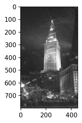
Is this pictuer of the
14.Terminal_Tower, 28.Sydney_Harbour_Bridge, 35.Monumento_a_la_Revolucion
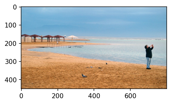
Is this pictuer of the
42.Death_Valley_National_Park, 18.Delicate_Arch, 03.Dead_Sea
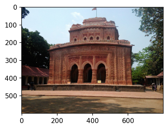
Is this pictuer of the
12.Kantanagar_Temple, 21.Taj_Mahal, 26.Pont_du_Gard
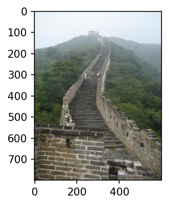
Is this pictuer of the
46.Great_Wall_of_China, 41.Machu_Picchu, 16.Eiffel_Tower
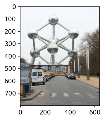
Is this pictuer of the
37.Atomium, 16.Eiffel_Tower, 42.Death_Valley_National_Park
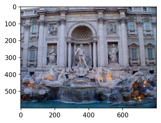
Is this pictuer of the
44.Trevi_Fountain, 32.Hanging_Temple, 40.Stockholm_City_Hall
