Human Resources Data Analysis

In this project, we embark on a journey of HR Analytics to analyze and visualize our company’s extensive dataset.
The multifaceted role of Human Resources professionals transcends the perceived simplicity of the job. HR experts engage in a spectrum of workplace activities, from spearheading recruitment efforts and resolving employee issues, to nurturing a positive work environment, and critically evaluating performance and efficiency.
Among their various duties, one of the most intricate tasks HR professionals face is the assessment of employee performance and efficiency. The complexity of this responsibility scales with the size of the employee base, posing a significant challenge to HR’s capability to manage effectively. In response to this challenge, we have initiated an Exploratory Data Analysis (EDA) project.
Within the scope of this project, we aim to conduct thorough analyses and create insightful visualizations using the Employee Engagement Dataset. Our objective is to derive valuable insights that can inform and refine HR practices. The project will dissect data on performance scores, scrutinize the link between performance and remuneration, investigate factors influencing employee attrition, and define the contours of employee satisfaction across different departments.
This analysis endeavors to arm HR professionals with robust data-driven insights, bolstering their ability to foster workforce development and support. By leveraging this strategic approach, we can enhance the impact and operational efficiency of HR functions.
This work is conducted under the dataset license “CC-BY-NC-ND: This work is licensed under a Creative Commons Attribution-NonCommercial-NoDerivatives 4.0 International License.” The license governs the use of the dataset, ensuring that it is utilized in a manner that aligns with the stipulated non-commercial and no-derivatives terms.
Import Necessary Libraries
First, let’s import the libraries that we will need.
import pandas as pd
import numpy as np
import matplotlib.pyplot as plt
import seaborn as sns
from datetime import datetime
Data Loading
Load the dataset into a Pandas DataFrame.
dataset = pd.read_csv('HRDataset_v14.csv')
dataset.info()
<class 'pandas.core.frame.DataFrame'>
RangeIndex: 311 entries, 0 to 310
Data columns (total 38 columns):
 #   Column                      Non-Null Count  Dtype
---  ------                      --------------  -----
 0   Employee_Name               311 non-null    object
 1   EmpID                       311 non-null    int64
 2   MarriedID                   311 non-null    int64
 3   MaritalStatusID             311 non-null    int64
 4   GenderID                    311 non-null    int64
 5   EmpStatusID                 311 non-null    int64
 6   DeptID                      311 non-null    int64
 7   PerfScoreID                 311 non-null    int32
 8   FromDiversityJobFairID      311 non-null    int64
 9   Salary                      311 non-null    int32
 10  Termd                       311 non-null    int64
 11  PositionID                  311 non-null    int32
 12  Position                    311 non-null    object
 13  State                       311 non-null    object
 14  Zip                         311 non-null    int64
 15  DOB                         311 non-null    datetime64[ns]
 16  Sex                         311 non-null    object
 17  MaritalDesc                 311 non-null    object
 18  CitizenDesc                 311 non-null    object
 19  HispanicLatino              311 non-null    object
 20  RaceDesc                    311 non-null    object
 21  DateofHire                  311 non-null    datetime64[ns]
 22  DateofTermination           104 non-null    datetime64[ns]
 23  TermReason                  311 non-null    object
 24  EmploymentStatus            311 non-null    object
 25  Department                  311 non-null    object
 26  ManagerName                 311 non-null    object
 27  ManagerID                   303 non-null    float64
 28  RecruitmentSource           311 non-null    object
 29  PerformanceScore            311 non-null    object
 30  EngagementSurvey            311 non-null    float64
 31  EmpSatisfaction             311 non-null    int64
 32  SpecialProjectsCount        311 non-null    int64
 33  LastPerformanceReview_Date  311 non-null    object
 34  DaysLateLast30              311 non-null    int64
 35  Absences                    311 non-null    int64
 36  Age                         311 non-null    int64
 37  Tenure                      311 non-null    int64
dtypes: datetime64[ns](3), float64(2), int32(3), int64(15), object(15)
memory usage: 88.8+ KB
dataset.head(5)
| Employee_Name | EmpID | MarriedID | MaritalStatusID | GenderID | EmpStatusID | DeptID | PerfScoreID | FromDiversityJobFairID | Salary | ... | RecruitmentSource | PerformanceScore | EngagementSurvey | EmpSatisfaction | SpecialProjectsCount | LastPerformanceReview_Date | DaysLateLast30 | Absences | Age | Tenure | |
|---|---|---|---|---|---|---|---|---|---|---|---|---|---|---|---|---|---|---|---|---|---|
| 0 | Adinolfi, Wilson K | 10026 | 0 | 0 | 1 | 1 | 5 | 4 | 0 | 62506 | ... | Exceeds | 4.60 | 5 | 0 | 1/17/2019 | 0 | 1 | 40 | 4528 | |
| 1 | Ait Sidi, Karthikeyan | 10084 | 1 | 1 | 1 | 5 | 3 | 3 | 0 | 104437 | ... | Indeed | Fully Meets | 4.96 | 3 | 6 | 2/24/2016 | 0 | 17 | 48 | 444 |
| 2 | Akinkuolie, Sarah | 10196 | 1 | 1 | 0 | 5 | 5 | 3 | 0 | 64955 | ... | Fully Meets | 3.02 | 3 | 0 | 5/15/2012 | 0 | 3 | 35 | 447 | |
| 3 | Alagbe,Trina | 10088 | 1 | 1 | 0 | 1 | 5 | 3 | 0 | 64991 | ... | Indeed | Fully Meets | 4.84 | 5 | 0 | 1/3/2019 | 0 | 15 | 35 | 5803 |
| 4 | Anderson, Carol | 10069 | 0 | 2 | 0 | 5 | 5 | 3 | 0 | 50825 | ... | Google Search | Fully Meets | 5.00 | 4 | 0 | 2/1/2016 | 0 | 2 | 34 | 1884 |
5 rows × 38 columns
dataset.describe()
| EmpID | MarriedID | MaritalStatusID | GenderID | EmpStatusID | DeptID | PerfScoreID | FromDiversityJobFairID | Salary | Termd | PositionID | Zip | ManagerID | EngagementSurvey | EmpSatisfaction | SpecialProjectsCount | DaysLateLast30 | Absences | Age | Tenure | |
|---|---|---|---|---|---|---|---|---|---|---|---|---|---|---|---|---|---|---|---|---|
| count | 311.000000 | 311.000000 | 311.000000 | 311.000000 | 311.000000 | 311.000000 | 311.000000 | 311.000000 | 311.000000 | 311.000000 | 311.000000 | 311.000000 | 303.000000 | 311.000000 | 311.000000 | 311.000000 | 311.000000 | 311.000000 | 311.000000 | 311.000000 |
| mean | 10156.000000 | 0.398714 | 0.810289 | 0.434084 | 2.392283 | 4.610932 | 2.977492 | 0.093248 | 69020.684887 | 0.334405 | 16.845659 | 6555.482315 | 14.570957 | 4.110000 | 3.890675 | 1.218650 | 0.414791 | 10.237942 | 44.408360 | 2915.569132 |
| std | 89.922189 | 0.490423 | 0.943239 | 0.496435 | 1.794383 | 1.083487 | 0.587072 | 0.291248 | 25156.636930 | 0.472542 | 6.223419 | 16908.396884 | 8.078306 | 0.789938 | 0.909241 | 2.349421 | 1.294519 | 5.852596 | 8.870236 | 1375.284534 |
| min | 10001.000000 | 0.000000 | 0.000000 | 0.000000 | 1.000000 | 1.000000 | 1.000000 | 0.000000 | 45046.000000 | 0.000000 | 1.000000 | 1013.000000 | 1.000000 | 1.120000 | 1.000000 | 0.000000 | 0.000000 | 1.000000 | 31.000000 | 26.000000 |
| 25% | 10078.500000 | 0.000000 | 0.000000 | 0.000000 | 1.000000 | 5.000000 | 3.000000 | 0.000000 | 55501.500000 | 0.000000 | 18.000000 | 1901.500000 | 10.000000 | 3.690000 | 3.000000 | 0.000000 | 0.000000 | 5.000000 | 37.000000 | 1812.500000 |
| 50% | 10156.000000 | 0.000000 | 1.000000 | 0.000000 | 1.000000 | 5.000000 | 3.000000 | 0.000000 | 62810.000000 | 0.000000 | 19.000000 | 2132.000000 | 15.000000 | 4.280000 | 4.000000 | 0.000000 | 0.000000 | 10.000000 | 43.000000 | 3304.000000 |
| 75% | 10233.500000 | 1.000000 | 1.000000 | 1.000000 | 5.000000 | 5.000000 | 3.000000 | 0.000000 | 72036.000000 | 1.000000 | 20.000000 | 2355.000000 | 19.000000 | 4.700000 | 5.000000 | 0.000000 | 0.000000 | 15.000000 | 50.000000 | 3794.000000 |
| max | 10311.000000 | 1.000000 | 4.000000 | 1.000000 | 5.000000 | 6.000000 | 4.000000 | 1.000000 | 250000.000000 | 1.000000 | 30.000000 | 98052.000000 | 39.000000 | 5.000000 | 5.000000 | 8.000000 | 6.000000 | 20.000000 | 72.000000 | 6531.000000 |
Data Preparation
Before we begin our analysis, let’s prepare our data by calculating the age of employees and ensuring data types are correct.
# Convert 'DOB' to datetime and calculate age
dataset['DOB'] = pd.to_datetime(dataset['DOB'])
current_year = datetime.now().year
dataset['Age'] = current_year - dataset['DOB'].dt.year

# Convert relevant columns to appropriate data types
dataset['PerfScoreID'] = dataset['PerfScoreID'].astype(int)
dataset['Salary'] = dataset['Salary'].astype(int)
dataset['PositionID'] = dataset['PositionID'].astype(int)
Data Visualization
Now, let’s create scatter plots to visualize the relationships between performance score and salary, age, and job level.
# Performance vs. Salary
plt.figure(figsize=(10, 5))
sns.scatterplot(data=dataset, x='PerfScoreID', y='Salary')
plt.title('Performance Score vs Salary')
plt.show()
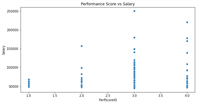
- The plot shows a series of discrete vertical clusters, corresponding to different performance scores.
- A positive correlation appears to be present, indicating that higher performance scores may be associated with higher salaries.
- The highest salaries are concentrated at the highest performance score (4.0), suggesting a possible reward system for top performers.
- There is a wide range of salaries within each performance score category, especially at the higher performance scores.
# Performance vs. Age
plt.figure(figsize=(10, 5))
sns.scatterplot(data=dataset, x='PerfScoreID', y='Age')
plt.title('Performance Score vs Age')
plt.show()
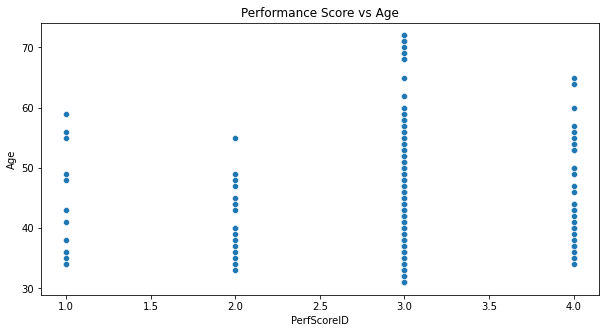
- The distribution of ages is relatively uniform across different performance scores.
- There doesn’t seem to be a clear trend or correlation between age and performance score, suggesting that performance may not be directly influenced by an employee’s age.
- Employees of a wide range of ages can be found at each performance score level, showing diversity in age among different performance categories.
# Performance vs. Job Level
plt.figure(figsize=(10, 5))
sns.scatterplot(data=dataset, x='PerfScoreID', y='PositionID')
plt.title('Performance Score vs Job Level')
plt.show()
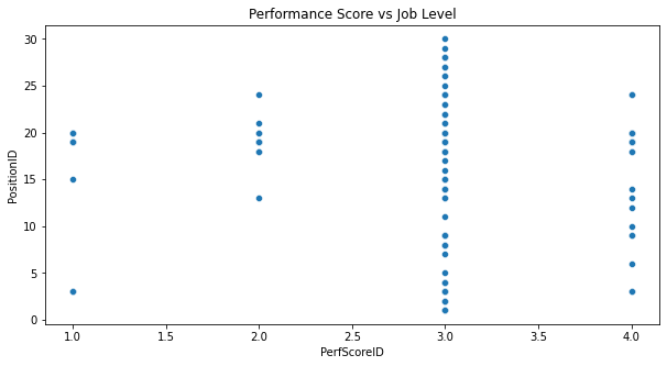
- Higher job levels appear more frequently at higher performance scores, suggesting a potential link between job level and performance.
- The most populated vertical cluster is at the highest performance score (4.0), which may indicate that higher job levels have a higher concentration of top performance ratings.
- There is a noticeable absence of lower job levels at the highest performance score, which could imply that such levels have a performance cap or that promotion to a higher job level is performance-dependent.
Overall, these plots suggest that while salary and job level have some association with performance scores, age does not show a significant relationship with performance. The findings indicate that the company might reward high performance with higher salaries and job levels, but performance evaluation is age-agnostic. These visual insights should be further investigated with statistical analyses to understand the strength and significance of these relationships.
Correlation Analysis
To quantify the relationships, we will calculate the correlation coefficients.
# Calculating correlation coefficients
salary_corr = dataset['PerfScoreID'].corr(dataset['Salary'])
age_corr = dataset['PerfScoreID'].corr(dataset['Age'])
job_level_corr = dataset['PerfScoreID'].corr(dataset['PositionID'])

# Print the correlation coefficients
print(f"Correlation between Performance Score and Salary: {salary_corr}")
print(f"Correlation between Performance Score and Age: {age_corr}")
print(f"Correlation between Performance Score and Job Level: {job_level_corr}")
Correlation between Performance Score and Salary: 0.1309025823175193
Correlation between Performance Score and Age: 0.07920301894181259
Correlation between Performance Score and Job Level: 0.005226508043668236
A correlation coefficient of 0.1309 indicates a positive but weak relationship between Performance Score and Salary. This suggests that while there may be a tendency for higher performance scores to correspond to higher salaries, the relationship is not strong. Many other factors likely contribute to determining salary that are not captured by performance score alone.
The correlation coefficient of 0.0792 is closer to zero, suggesting a very weak positive relationship between Performance Score and Age. This aligns with the visual observation from the scatter plot, where age did not appear to have a significant impact on performance score. Performance seems to be relatively independent of age.
With a correlation coefficient of 0.0052, there is virtually no linear relationship between Performance Score and Job Level. This coefficient is very close to zero, which suggests that job level does not predict performance score and vice versa, at least not linearly. This might be surprising given the visual cluster of higher job levels at the top performance score, but it indicates that across all job levels, performance scores are varied and not systematically higher with increasing job level.
These correlation coefficients highlight the importance of considering multiple factors when analyzing employee performance and compensation. Although there may be a perceived relationship, the actual correlation may be weak, emphasizing that performance scores are influenced by a complex interplay of various factors beyond just salary, age, or job level.
Employee Satisfaction Levels Across Different Departments
Let’s examine if there’s a difference in employee satisfaction levels across various departments.
Data Visualization
# Grouping by Department and calculating average satisfaction
department_satisfaction = dataset.groupby('Department')['EmpSatisfaction'].mean()

# Creating a bar chart with figure size specified for better visibility
plt.figure(figsize=(12, 6))
bars = plt.bar(department_satisfaction.index, department_satisfaction.values)

# Adding the value labels on top of the bars
for bar in bars:
    yval = bar.get_height()
    plt.text(bar.get_x() + bar.get_width()/2, yval + 0.05, round(yval, 2), ha='center', va='bottom')

plt.title('Average Employee Satisfaction by Department')
plt.ylabel('Average Satisfaction')
plt.xticks(rotation=45, ha='right')  # Rotate labels to avoid overlap
plt.show()
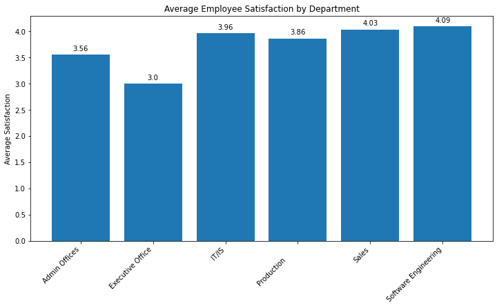
- All departments have a relatively high level of average employee satisfaction, with all scores above 3.0 on a scale that appears to go up to 4.0.
- The Admin Offices have the lowest average satisfaction score among the five departments, but the score is still above 3.0, indicating generally positive satisfaction.
- The Executive Office has a slightly higher average satisfaction score than the Admin Offices but is still lower than the other three departments.
- IT/IS, Production, and Software Engineering departments have very similar levels of average employee satisfaction, all close to 4.0, which suggests that employees in these departments are the most satisfied overall.
- The Software Engineering department has the highest average satisfaction score, albeit by a narrow margin.
Based on this chart, one can conclude that while employee satisfaction is generally high across the company, there are slight variations between departments. The reasons behind the lower satisfaction in the Admin Offices compared to the other departments could be a point of interest for further investigation. Additionally, the factors contributing to the high satisfaction in Software Engineering might be explored for potential adoption in other departments.
Job Level and Likelihood to Leave the Company
We will investigate how an employee’s job level relates to their likelihood of leaving the company.
Data Analysis and Visualization
# Calculating attrition rate by job level
attrition_rate = dataset[dataset['Termd'] == 1].groupby('PositionID').size() / dataset.groupby('PositionID').size()

# Creating a bar chart
plt.figure(figsize=(10, 5))
attrition_rate.plot(kind='bar')
plt.title('Attrition Rate by Job Level')
plt.ylabel('Attrition Rate')
plt.show()
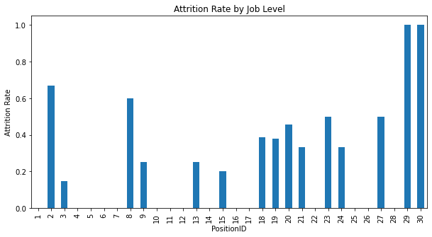
- The attrition rate varies significantly across different job levels.
- Lower job levels (as indicated by the lower PositionID numbers) generally have lower attrition rates, with some fluctuation.
- As the PositionID increases, indicating higher job levels, there is a general trend of increasing attrition rate, with some positions having notably higher rates than others.
- The highest attrition rate is seen at the highest PositionID shown on the chart, which is nearly 1.0. This could suggest that employees at this job level are either all or almost all leaving the company.
Based on these observations, it can be inferred that job level may be a factor in an employee’s decision to stay with or leave the company. The reasons behind the higher attrition rate at the highest job level could be varied, ranging from career advancement opportunities elsewhere to possible dissatisfaction or restructuring at higher organizational levels. It may be beneficial for the company to investigate the specific causes of attrition at higher job levels to develop strategies to retain key talent.
Impact of Tenure on Salary and Performance Rating
Next, we’ll explore how the length of time an employee has been with the company impacts their salary and performance rating.
Data Preparation
# Calculate tenure
dataset['DateofHire'] = pd.to_datetime(dataset['DateofHire'])
dataset['DateofTermination'] = pd.to_datetime(dataset['DateofTermination'])
dataset['Tenure'] = dataset.apply(lambda x: (x['DateofTermination'] - x['DateofHire']).days if pd.notna(x['DateofTermination']) else (datetime.now() - x['DateofHire']).days, axis=1)
Data Visualization
# Tenure vs. Salary
plt.figure(figsize=(10, 6))
sns.scatterplot(data=dataset, x='Tenure', y='Salary')
plt.title('Tenure vs Salary')
plt.show()
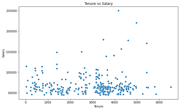
- The plot shows a wide range of salaries across different tenure lengths.
- There is no distinct upward trend that suggests a strong positive correlation between tenure and salary. While some employees with longer tenure have higher salaries, there is considerable variation, and some long-tenured employees have salaries similar to those with shorter tenures.
- There are several outliers, particularly employees with higher salaries, which do not follow a clear trend related to tenure.
- The majority of data points are clustered at the lower end of the salary spectrum, regardless of tenure.
# Tenure vs. Performance Score
plt.figure(figsize=(10, 6))
sns.scatterplot(data=dataset, x='Tenure', y='PerfScoreID')
plt.title('Tenure vs Performance Score')
plt.show()
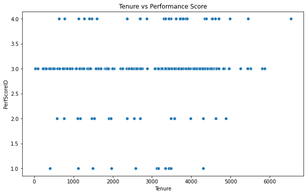
- Performance scores are distributed across various tenure lengths with a large concentration of scores around the 3.0 mark.
- There is no clear trend indicating that longer tenure results in higher performance scores. Performance scores seem to be consistent across different tenure lengths.
- There is a ceiling effect visible with performance scores, where scores do not exceed 4.0. This could be the maximum score achievable in the performance rating system.
- The distribution suggests that performance evaluations are not directly tied to the length of tenure, as employees with varying lengths of tenure have similar performance scores.
These findings suggest that while there may be some relationship between tenure and salary, it is not strongly linear, and other factors likely play a significant role in determining salary. Similarly, tenure does not appear to be a strong predictor of performance score. This could imply that the company’s performance evaluations are based on criteria other than tenure, or that employees reach a performance plateau regardless of how long they have been with the company.
Reasons for Employee Attrition and Patterns
Finally, we’ll look at the most common reasons for employee attrition and see if there are any patterns based on age, tenure, or performance rating.
Data Visualization for Reasons of Attrition
# Counting the reasons for attrition
attrition_reasons = dataset[dataset['Termd'] == 1]['TermReason'].value_counts()

# Creating a bar chart
plt.figure(figsize=(10, 5))
attrition_reasons.plot(kind='bar')
plt.title('Reasons for Employee Attrition')
plt.xlabel('Reasons')
plt.ylabel('Frequency')
plt.xticks(rotation=45, ha='right')  # Rotate labels to avoid overlap
plt.show()
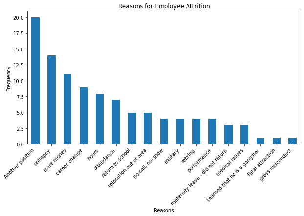
- The most common reason for employee attrition is another position, indicating that a significant number of employees leave for jobs at other companies.
- The second most frequent reason is unhappy, suggesting that job dissatisfaction is a major factor in employees’ decision to leave.
- More money and career change follow as the next most common reasons, which could imply that financial incentives and professional growth opportunities elsewhere are influencing factors in attrition.
- Other notable reasons include hours, attendance, and return to school, but these are less frequent compared to the top reasons.
- Reasons such as medical issues, relocating out of area, military, retiring, maternity leave - did not return, performance, and no-call, no-show are the least common, indicating that they are not the primary drivers of employee turnover in this dataset.
- The variety of reasons suggests that attrition is a multifaceted issue, with a range of personal and professional factors contributing to employees’ decisions to leave.
These insights can help the company address the underlying causes of attrition. For example, improving job satisfaction and offering competitive compensation may reduce turnover. Additionally, providing clear career progression paths could potentially retain employees looking for a career change. Understanding these reasons in more depth could guide targeted retention strategies.
Analyzing Patterns of Attrition
# Attrition by Age
plt.figure(figsize=(10, 6))
sns.boxplot(x='Termd', y='Age', data=dataset)
plt.title('Attrition by Age')
plt.show()
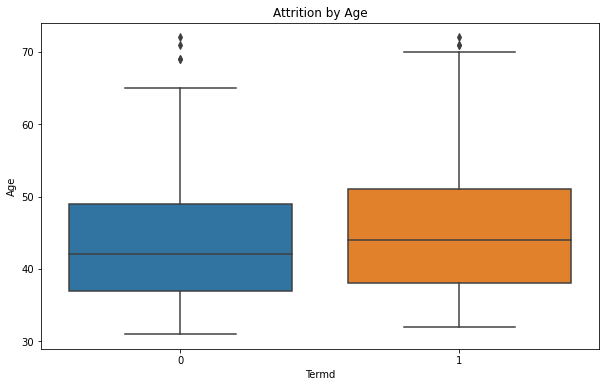
- The age range of employees who have not left the company (Termd = 0) is slightly lower with a median age around the late 40s.
- The age distribution for those who have left the company (Termd = 1) is broader, with a higher median age around the early 50s.
- There are outliers in both categories, with some older employees who have not left the company and some who have.
# Attrition by Tenure
plt.figure(figsize=(10, 6))
sns.boxplot(x='Termd', y='Tenure', data=dataset)
plt.title('Attrition by Tenure')
plt.show()
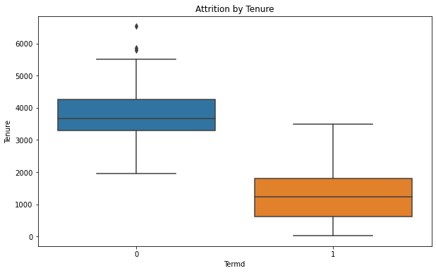
- Employees who have not left the company tend to have a wide range of tenure, with a median tenure that appears to be around 3000 days, suggesting long-term employment.
- The tenure of employees who have left is generally lower, with a median around 2000 days, indicating they leave the company earlier in their tenure.
- The range of tenure is narrower for those who have left, which suggests there’s less variability in tenure among employees who decide to leave.
# Attrition by Performance Score
plt.figure(figsize=(10, 6))
sns.boxplot(x='Termd', y='PerfScoreID', data=dataset)
plt.title('Attrition by Performance Score')
plt.show()
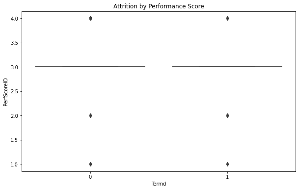
- The performance scores for employees who have not left the company are distributed mostly at the higher end of the scale, with the median score close to 3.0.
- For employees who have left, the performance scores are also high, with a median score similar to those who haven’t left, which suggests that performance scores alone are not a strong predictor of whether an employee will leave.
- There are a few outliers on both sides, indicating some employees with lower performance scores have not left, and some with higher scores have left.
Overall, these box plots suggest that age and tenure may have some influence on attrition, with employees who are older and have shorter tenure being more likely to leave. Performance score does not appear to be a decisive factor in attrition, as scores are relatively high for both those who have and have not left the company. It’s important to note that box plots show the distribution of a dataset and can reveal the central tendency and dispersion, but they do not demonstrate causation. Further analysis would be necessary to understand the reasons behind these trends.
In conclusion, while performance seems to be recognized in terms of salary to some degree, there are clear indications that the company might benefit from examining its compensation strategies, job satisfaction drivers, and career development opportunities to address attrition causes. The lack of strong correlation between performance and job level suggests that career progression might not be entirely merit-based or that the evaluation system spreads scores evenly across roles. Addressing these findings could lead to improved employee retention, better job satisfaction, and a more transparent and effective performance evaluation system.